ResNet: Residuals Make Depth Trainable, but ImageNet 2015 Is Not a Ready-Made Detection or ViT Contract

Pair this with the three-pass approach. In this site’s sequence of foundational CV methods, this note follows AlexNet part 1 and part 2. AlexNet shows that a large CNN can be trained effectively on ImageNet; ResNet asks why deeper plain nets get worse and how identity shortcuts rewrite the optimization problem.

The paper in 90 seconds

• Problem: After batch normalization and good initialization made tens of layers trainable, stacking more plain conv layers still triggers degradation—deeper models show higher training error (Figure 1, Figure 4 left), which is not ordinary overfitting.
• Core insight: Recast the target mapping. Instead of asking stacked nonlinear layers to fit $\mathcal{H}(\mathbf{x})$ directly, let them fit $\mathcal{F}(\mathbf{x}):=\mathcal{H}(\mathbf{x})-\mathbf{x}$ and output $\mathbf{y}=\mathcal{F}(\mathbf{x})+\mathbf{x}$ through identity shortcuts (Equation 1). The control point is whether the solver must fit $H(x)$ from scratch or learn a correction $F(x)$ on top of identity.
• Strongest evidence: On ImageNet with matched parameter counts, plain-34 top-1 error is 28.54% versus plain-18 27.94%, while ResNet-34 is 25.03% and beats ResNet-18 27.88% (Table 2, 10-crop validation). On CIFAR-10, plain-56 training error exceeds 60% and is omitted from Figure 6 left, while ResNet depth scans down to ResNet-110 6.43% (Table 6, Figure 6). ResNet-152 single-model top-5 validation error is 4.49%; a six-model ensemble reaches 3.57% top-5 on test (Tables 4–5).
• Main boundary: The headline contract is 2012 ImageNet classification plus CIFAR-10 depth diagnostics; PASCAL/COCO detection is a Faster R-CNN backbone transfer table (Tables 7–8), not a YOLO contract, not ViT, and not a modern ConvNet leaderboard.

My conclusion: ResNet’s most useful contribution is making deeper networks easier to optimize through identity shortcuts and residual mappings. The ILSVRC 2015 ensemble result of 3.57% and the COCO mAP results are not specifications for today’s detection or Transformer systems.

Version and reading scope

This note reads He et al., CVPR 2016 against arXiv:1512.03385 v1 (first posted 2015-12-10). The PDF is marked with the arXiv.org perpetual non-exclusive license; the CVPR camera-ready is additionally under IEEE terms. Author order follows the v1 PDF: Kaiming He, Xiangyu Zhang, Shaoqing Ren, and Jian Sun at Microsoft Research.

Beyond the abstract, the note checks Section 3’s residual formulation and architectures, Section 3.4 training, Section 4.1 ImageNet classification (Tables 1–5, Figures 3–5), Section 4.2 CIFAR-10 (Table 6, Figures 6–7), Section 4.3 detection transfer (Tables 7–8), and artifact endpoints as of 2026-08-28. YOLO mAP, ViT accuracy, and ConvNeXt / ResNet-RS numbers are not written back.

This is a published CVPR paper, not a preprint-only story.

The question the reader actually needs

Once you can train an AlexNet-scale CNN, should you keep stacking plain layers for more representational depth, or change the optimization target? He et al. answer: insert parameter-free identity shortcuts into a VGG-style plain backbone so each block learns $\mathcal{F}(\mathbf{x})+\mathbf{x}$ instead of an unreferenced $\mathcal{H}(\mathbf{x})$.

The precise reading is not “is ResNet the 2026 default backbone?” The real question is: does residual learning remove degradation, where does depth pay off, and which numbers are 2015 classification evidence versus detection transfer?

Evidence map

Layer	How this article uses it
Paper directly supports	Figures 1 / 6 left: deeper plain nets raise training and test error; Figures 4 right / 6 middle: deeper ResNets lower error. Figure 2 defines the block; Figure 3 contrasts VGG-19, plain-34, and ResNet-34. Table 2 compares matched plain vs ResNet; Tables 3–4 depth variants; Table 6 CIFAR depth scan; Figure 7 smaller residual branch responses.
Author claims	Residual learning eases degradation; very deep ResNets optimize and gain from depth; identity shortcuts are enough and cheap; the principle generalizes to detection/segmentation in competition narratives.
Not established	“Deeper is always better” on every task; 1202 layers beat 110 on CIFAR test; the best modern optimizer/regularization recipe; mechanical bottleneck copying in the ViT era; detection tables as today’s object-detector contract.
Bloss0m engineering judgment	Place this paper after the AlexNet pair in the sequence of foundational CV methods. COCO mAP and ILSVRC 2015 ensemble scores should not be mixed into later YOLO or ViT notes.

Later sections keep numbers, author claims, and engineering judgment apart. “SOTA” means the row in the paper’s tables at writing time, not a 2026 leaderboard.

Why the previous approach is insufficient

Section 1 sets the stage. AlexNet (part 1) and later VGG / GoogLeNet showed depth helps; vanishing gradients were eased by normalized initialization and batch normalization, letting networks with tens of layers start converging.

Stacking further still exposed degradation: accuracy saturates then collapses, and training error rises with depth (Figure 1’s 20 vs 56 plain layers on CIFAR-10; Figure 4 left’s 18 vs 34 plain layers on ImageNet). The issue is not memorizing the training set—it is that solvers struggle to find solutions no worse than a shallower net, even though a deeper model could in principle implement “extra identity layers + copy shallow weights.”

The AlexNet pair teaches capacity, ReLU, augmentation, and regularization for an eight-layer-scale system; it does not fix the optimization floor of 30+ plain layers. ResNet changes the block-level objective, not a new activation gimmick.

Core intuition

Ignore the ImageNet leaderboard for a moment. You append 16 layers after an 18-layer trunk. If the new layers should ideally do nothing, the simplest map is identity. Plain nonlinear stacks struggle to learn identity; the solver instead raises training error.

ResNet says the new layers should output only a correction $\mathcal{F}(\mathbf{x})$ relative to input $\mathbf{x}$, with $\mathbf{x}$ carried by a shortcut. If the optimum is near identity, driving $\mathcal{F}$ toward zero is easier than teaching conv layers identity from scratch. Figure 7 shows residual branch response standard deviations smaller than plain nets, supporting “corrections are usually small.”

Contrast three next steps that later writing often collapses:

• Plain deep CNN (VGG style): each block must re-encode all of $\mathcal{H}(\mathbf{x})$ with no reference shortcut.
• ResNet (this paper): block output is $\sigma(\mathcal{F}(\mathbf{x})+\mathbf{x})$; matched-dimension shortcuts add no parameters and no extra FLOPs (Section 3.2).
• Later methods (ViT, ConvNeXt, and one-stage detectors): change tokenization, stage design, or task heads; Table 5’s 3.57% does not belong to those systems.

Walk one example through the method

The walk uses Figure 2’s two-layer residual block on an ImageNet conv feature map, not a standalone experiment ID.

1. Input: feature map $\mathbf{x}$ with the same channels and spatial size as the previous block output (for example 28×28 with 128 channels in conv3_x).
2. Intermediate representation: main path computes $\mathcal{F}(\mathbf{x})=W_2\,\mathrm{ReLU}(W_1\mathbf{x})$ (two 3×3 convs, Figure 2); the shortcut passes $\mathbf{x}$ unchanged.
3. Model or system decision: element-wise sum yields $\mathbf{y}=\mathcal{F}(\mathbf{x})+\mathbf{x}$, then ReLU. When dimensions change (dotted shortcuts in Figure 3), use zero-padding (option A) or a 1×1 projection $W_s\mathbf{x}$ (option B, Equation 2); Table 3 shows A/B/C all far above plain nets, so identity is already enough.
4. Output: $\mathbf{y}$ feeds the next residual block; the full network ends with global average pooling plus a 1000-way fc layer (Section 3.3).
5. Likely failure point: blind depth on small data—the 1202-layer CIFAR ResNet reaches training error below 0.1% but test error 7.93%, worse than the 110-layer 6.43% (Table 6, Figure 6 right); the authors attribute this to overfitting, not optimization failure. Another failure mode is reading the wrong evidence domain: treating COCO +6.0 mAP as a guarantee for your classification head design.

Technical mechanism

Residual block

Equation (1):

$$\mathbf{y}=\mathcal{F}(\mathbf{x},\{W_i\})+\mathbf{x}.$$

When dimensions mismatch, use the projection shortcut in Equation (2). A single-layer $\mathcal{F}$ collapses to a linear additive form; the authors report no advantage (Section 3.2).

Network family (Table 1, Figures 3 and 5)

• Plain baseline: VGG philosophy—3×3 convs, constant channels per resolution, double channels when halving spatial size; 34-layer plain is about 3.6×10⁹ FLOPs, only 18% of VGG-19.
• ResNet-18/34: two 3×3 basic blocks.
• ResNet-50/101/152: three-layer bottlenecks (1×1 down → 3×3 → 1×1 up, Figure 5). The 152-layer model is about 11.3×10⁹ FLOPs, still below VGG-16/19.

Training and evaluation (Section 3.4)

ImageNet: random scale with shorter side in $[256,480]$, 224 crops, color augmentation, BN after each conv, no dropout. SGD batch 256, learning rate 0.1 (divide by 10 on plateau), up to 60×10⁴ iterations, weight decay 0.0001, momentum 0.9. Testing uses 10-crop; best numbers average multi-scale fully convolutional scores.

CIFAR-10 (Section 4.2): 6n+2 layer stacks, batch 128 on two GPUs; learning rate 0.1 with divides at 32k and 48k, training ends at 64k iterations. The 110-layer model warms up at 0.01 until training error drops below 80%, then returns to 0.1.

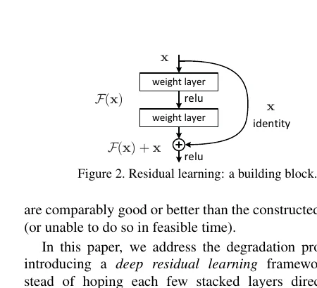
Figure 2, Section 3.2: the building block matching Equation (1). Locatable at arXiv PDF Figure 2. Cropped from the CVPR 2016 camera-ready PDF; copyright remains with the authors/IEEE. This note preserves attribution for scholarly commentary and cites arXiv reuse terms.

How to read the evidence

Figures 1 and 4: degradation and its reversal

Question: Does a deeper plain net optimize better? Controls: CIFAR-10 20 vs 56 layers (Figure 1); ImageNet 18 vs 34 plain layers (Figure 4 left). Observation: deeper curves show higher training and validation error. Boundary: this is an optimization diagnostic, not the final ImageNet leaderboard.

Matched-depth ResNets reverse the picture (Figure 4 right): ResNet-34 training error falls below ResNet-18 and far below plain-34. Table 2 quantifies: plain-34 top-1 28.54% versus ResNet-34 25.03% (a 3.51 point gap), while plain-34 is 0.60 points worse than plain-18.

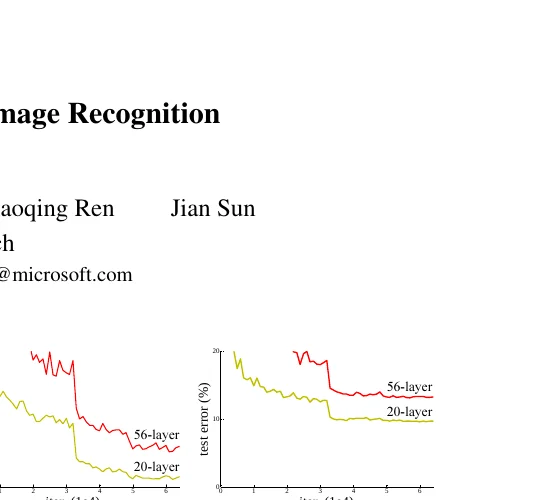
Figure 1, Introduction: left training error, right test error. See arXiv PDF Figure 1. Crop and license note match Figure 2.

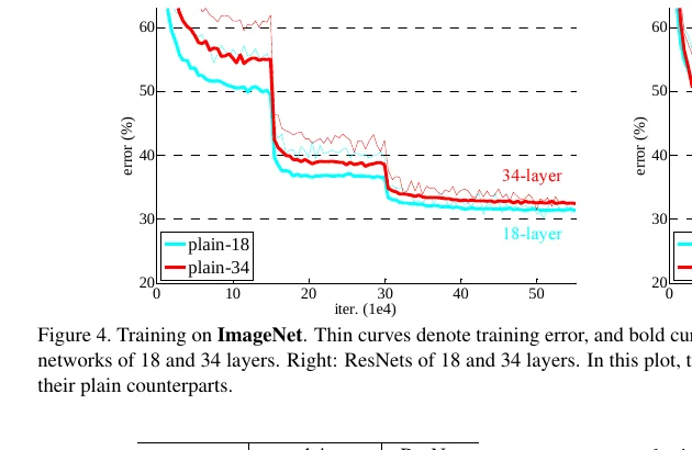
Figure 4, Section 4.1: thin curves training, bold curves validation center crops. See arXiv PDF Figure 4. Crop and license note match Figure 2.

Tables 3–4: depth variants and single-model classification

Question: Beyond 34 layers, do bottleneck ResNets keep improving? Observation (10-crop validation, Table 3): ResNet-50 top-1 22.85%, 101 21.75%, 152 21.43%; top-5 errors 6.71% / 6.05% / 5.71%. Table 4’s best single model: ResNet-152 top-1 19.38%, top-5 4.49%.

Boundary: these are ILSVRC 2012 validation classification errors under 10-crop and multi-scale protocols—not COCO detection mAP, not ViT numbers on JFT.

Table 5: ensemble and competition narrative

A six-model ensemble of different depths reaches 3.57% top-5 error on test (Table 5), the ILSVRC 2015 classification winning entry. Teach Table 4 single-model numbers separately: 3.57% is ensemble plus test-server reporting, not the error budget of deploying one ResNet-152.

Table 6 / Figures 6–7: CIFAR depth scan and mechanism diagnostics

Question: Is the phenomenon ImageNet-specific? Observation: plain 56-layer CIFAR error exceeds 60% (Figure 6 left, not plotted); ResNet-20 through 110 moves from 8.75% down to 6.43% (Table 6). The 1202-layer model trains (training error below 0.1%) but tests at 7.93%, worse than 110 layers—an overfitting boundary case.

Figure 7: ResNet layer response standard deviations are smaller than plain nets, and deeper ResNets perturb signals less per layer. This supports the residual motivation; it is not an extra accuracy claim.

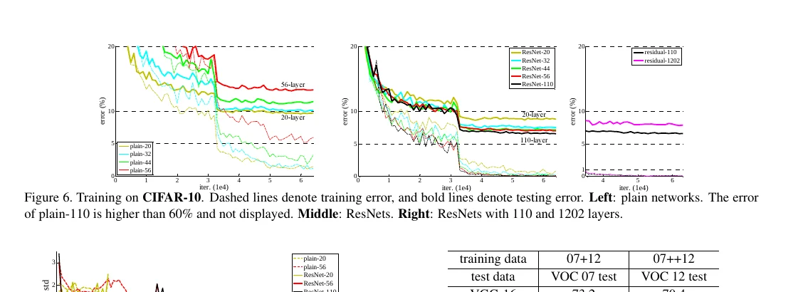
Figure 6, Section 4.2: dashed training, solid test. See arXiv PDF Figure 6. Crop and license note match Figure 2.

Tables 7–8: detection transfer (secondary, not the headline)

With Faster R-CNN, swapping the backbone gives COCO val mAP@[.5,.95] 27.2% for ResNet-101 versus 21.2% for VGG-16 (+6.0 absolute, 28% relative, Section 4.3). The authors argue representations improved, but the experiment is a detection baseline, independent of the classification tables.

Bloss0m judgment: memorize Tables 2–4 first; treat Tables 7–8 as a footnote that features transfer—do not promote them to YOLO or ViT teaching evidence.

Ablations and design choices

• Identity vs projection (Table 3 A/B/C): all shortcut types crush plain nets; B slightly beats A, C slightly beats B but adds thirteen projection shortcuts and complexity. The paper mainly adopts option B and stresses identity for bottlenecks (otherwise FLOPs roughly double).
• Matched-parameter fairness (Table 2): compared ResNets and plain nets share parameter counts (option A zero-padding), ruling out “just wider” explanations.
• Non-bottleneck depth (Figure 5 footnote): deeper non-bottleneck ResNets still gain on CIFAR, but bottlenecks are more economical.

Limitations and threats to validity

1. Era and data: ImageNet 2012 and CIFAR-10 are not modern data distributions or self-supervised pretraining.
2. Evaluation protocol: 10-crop, multi-scale, ensemble, and competition test numbers must not be merged.
3. Extreme depth is not automatically better: the 1202-layer CIFAR counterexample; the paper deliberately skips maxout/dropout-style heavy regularization (Section 4.2).
4. Detection/segmentation: multi-track competition wins are narrative context; engineering still needs an independent read of the detection pipeline—classification 3.57% does not imply a detection mAP contract.
5. Keep evidence scopes separate: YOLO, ViT, Swin, ConvNeXt, and ResNet-RS numbers and design choices are outside this PDF’s tables.
6. Versus Highway nets (Section 2): Highway uses gated, parameterized shortcuts that can close; ResNet identity shortcuts never close and always pass $\mathbf{x}$ while learning residuals.

Engineering decision and when not to use it

When to borrow this paper: you are deepening a vision backbone and see training loss worsen with depth (degradation). Check for missing skip/residual paths before blindly adding regularization or shaving depth. Default to identity shortcuts when dimensions match; use 1×1 projection only for channel/stride changes.

When not to copy it wholesale:

• Your task is one-stage detection or ViT classification—ResNet table numbers are not your contract; remeasure on your pipeline.
• Your dataset is tiny (CIFAR-scale) but you chase thousand-layer stacks—read the 1202-layer counterexample first.
• You embed ILSVRC 2015 ensemble 3.57% in a product SLA.
• You need minimum latency—a 152-layer bottleneck is not free; measure FLOPs on your hardware.

Huahua’s judgment

From AlexNet, keep separating architecture, training, and evidence boundaries; from ResNet, add one more rule—prove the optimization problem changed before assuming deeper is better.

Artifacts and reproducibility

As of 2026-08-28, direct endpoint status:

• Paper: arXiv abs and PDF are readable; CVF open-access HTML opens. Licensing follows arXiv and IEEE terms.
• Code: KaimingHe/deep-residual-networks (Caffe) returns HTTP 200 as a usable historical artifact; it is not a one-click PyTorch reproduction of Table 4 training logs. Modern implementations (torchvision resnet*, and others) are downstream ports, not identical to the original training run.
• Data: ImageNet 2012 requires a license; ILSVRC test labels are not public. CIFAR-10 is public but uses different hyperparameters than ImageNet.
• Microsoft Research project page: the microsoft.com publication URL returns 403 in this environment; do not claim extra artifacts from it.

A minimal useful reproduction: load ResNet-34 in torchvision or equivalent and compare training curves of plain versus residual stacks on a small image classification task—validate the mechanism, not 3.57%.

Three things to remember

1. Technical idea: identity shortcuts rewrite layer outputs as $\mathcal{F}(\mathbf{x})+\mathbf{x}$ so the solver learns residuals instead of unreferenced maps—the control point that makes depth trainable.
2. Evidence: plain-34 is worse than plain-18 (28.54% vs 27.94% top-1) while ResNet-34 is 25.03% and beats ResNet-18; CIFAR and Figure 7 support the mechanism story; ResNet-152 single-model top-5 is 4.49%, with ensemble test 3.57% kept separate.
3. Boundary: this is 2015–16 ImageNet classification plus CIFAR depth diagnostics; COCO mAP is transfer evidence, not a YOLO or ViT contract. AlexNet teaches that large CNNs can train; ResNet teaches how to rewrite the problem when depth increases.

Further reading

If you have not read the starting point for these foundational CV methods, return to AlexNet part 1 and part 2; for the reading method, see the three-pass approach. The next paper, original YOLO, covers unified real-time detection. Transformer-based methods address different questions and remain outside this note’s scope.

Primary sources

• He et al., “Deep Residual Learning for Image Recognition,” CVPR 2016 / arXiv:1512.03385 v1
• CVF open-access camera-ready
• DOI 10.1109/CVPR.2016.90
• KaimingHe/deep-residual-networks (Caffe)