AlexNet Part 2: Turning the Training Recipe into Testable Design Choices

The paper in 90 seconds

• Problem: In 2012, training a deep convolutional neural network with 60 million parameters and 650,000 neurons on ImageNet’s 1.2 million labeled images was constrained by crippling overfitting; simultaneously, saturating activation functions and the 3GB VRAM ceiling of desktop GPUs made backpropagation prohibitively slow or impossible to execute on a single chip.
• Core insight: AlexNet’s true breakthrough was not merely depth, but integrating non-saturating non-linearities (ReLU), multi-GPU split topology, label-preserving geometric and photometric data augmentation, hidden-unit dropout, and stochastic gradient descent with momentum into an interdependent, trainable systems engineering recipe.
• Strongest evidence: PCA color perturbation reduced top-1 error by over 1%, overlapping pooling reduced top-1 and top-5 error by 0.4% and 0.3%, and ReLU enabled a four-layer CNN on CIFAR-10 to reach 25% training error six times faster than $\tanh$; the complete system achieved 37.5% top-1 and 17.0% top-5 error on ILSVRC-2010, winning the 2012 competition with 15.3% top-5 compared to 26.2% for the second-place entry (Sections 3–6; Table 1).
• Main boundary: The paper’s diagnostic numbers represent single-component comparisons rather than a full factorial ablation; local response normalization (LRN), cross-GPU channel grouping, and test-time 10-crop ensembling were shaped by period-specific hardware limits and must not be imported unquestioningly as modern defaults.

This reading follows the official paper published in the NeurIPS 2012 proceedings (“ImageNet Classification with Deep Convolutional Neural Networks”). Continuing from AlexNet Part 1 on problem framing, evaluation protocols, and macro-architecture, this second part focuses on internal layer connectivity, regularization mechanics, numerical optimization dynamics, and reproducibility boundaries.

Huahua’s Engineering Note

Many assume AlexNet’s historical triumph was simply “stacking eight convolutional layers,” but in production engineering, a deep network that fails to converge or catastrophically overfits has zero value. AlexNet’s lasting legacy is decomposing “how to maintain gradient flow (ReLU),” “how to fit inside constrained hardware (dual-GPU splitting),” and “how to force high capacity to generalize (augmentation and Dropout)” into measurable, testable engineering hypotheses.

What to know first

In 2012, before deep learning became standard across computer vision, training large-scale convolutional networks faced several fundamental barriers. To understand why previous approaches were insufficient, consider these key bottlenecks:

1. Expressive capacity limits of traditional shallow methods: Prior state-of-the-art vision pipelines relied on handcrafted visual features (such as SIFT and HOG) paired with spatial encoding schemes (like Fisher Vectors or Sparse Coding) and linear support vector machines (SVMs). These traditional approaches plateaued when handling the intra-class diversity of ImageNet’s 1,000 fine-grained categories and failed to scale effectively with raw data volume.
2. Gradient vanishing from saturating activation functions: Classic artificial neural networks overwhelmingly utilized saturating non-linearities such as Sigmoid $f(x) = (1 + e^{-x})^{-1}$ or hyperbolic tangent $\tanh(x) = (e^x - e^{-x})/(e^x + e^{-x})$. As the magnitude of input $|x|$ grows, the derivative drops rapidly toward zero ($\tanh'(x) \to 0$). During backpropagation across multiple layers, chained multiplication of vanishing derivatives halted weight updates in earlier convolutional layers, making training deep models intolerably slow.
3. Hardware memory bottlenecks on desktop accelerators: In 2012, top-tier consumer GPUs (NVIDIA GeForce GTX 580) offered only 3GB of on-board memory. Storing forward activation maps, backward gradient tensors, optimizer states, and 60 million floating-point parameters exceeded single-GPU capacity. Without an explicit multi-GPU partitioning scheme, the model could not run.
4. Catastrophic overfitting between model capacity and training data: With 60 million parameters and 650,000 neurons, the network possessed vast expressive freedom. Even across ImageNet’s 1.2 million training images, training purely on fixed center crops allowed the network to memorize training instances; simultaneously, training an ensemble of separate deep networks was computationally out of reach.

The central dilemma of earlier work was clear: vision tasks required massive parameter capacity to model visual complexity, yet practitioners lacked systematic mechanisms to make deep models converge in practical wall-clock time without catastrophic overfitting.

Core intuition

The core intuition of AlexNet Part 2 is unambiguous: Deep neural network capacity is not an isolated mathematical artifact; training success depends on the system synergy of optimization velocity, hardware memory layout, continuous data distribution expansion, and implicit ensembling.

Prior practice operated on the conservative decision rule: “Use saturating activations to prevent activations from exploding, rely on basic L2 weight decay and early stopping, and limit model size to fit single-chip memory.” AlexNet inverted this into four actionable engineering principles:

1. Replace saturating activations with non-saturating piecewise linear units: Rectified Linear Units (ReLU) $f(x) = \max(0, x)$ maintain a constant derivative of 1 for all positive inputs, eliminating gradient saturation and speeding up gradient descent by an order of magnitude;
2. Replace global synchronization with asymmetric inter-GPU communication: Manually partition kernels across two GPUs, restricting communication to specific intermediate and classifier layers to trade communication bandwidth for feature capacity;
3. Expand the effective empirical distribution via label-preserving transformations: Apply real-time spatial crops, horizontal reflections, and PCA-based illumination jittering to transform static training examples into a continuous distribution;
4. Approximate exponential sub-network ensembling via stochastic masking: Use Dropout on fully connected layers to simulate a weight-sharing ensemble of astronomical scale at single-network training cost, breaking fragile co-adaptations between neurons.

Walk one example through the method

To trace AlexNet’s full training and inference lifecycle, walk a single image labeled “Siberian husky” through five sequential execution phases:

1. Input and label-preserving transformations: The raw image possesses arbitrary aspect ratios. The data pipeline rescales the shorter dimension to 256 pixels and crops the center $256 \times 256$ region. During training, CPU worker threads extract a random $224 \times 224$ patch on the fly, horizontally flip it with 50% probability, and inject an RGB offset calculated from the dataset-wide PCA covariance matrix. The original static photograph is thus transformed into an altered training variant without altering the ground-truth label.
2. Intermediate representation and split topology: The augmented $224 \times 224 \times 3$ patch enters the first convolutional layer (Conv1). 96 kernels of size $11 \times 11 \times 3$ are split evenly across two GPUs (48 kernels per GPU). In the subsequent Conv2 layer, kernels on each GPU process only the feature maps produced on the same GPU. Only at Conv3 do the two GPUs cross-communicate, sharing all 256 feature maps to build integrated higher-level representations, before reverting to local computation in Conv4 and Conv5.
3. Decision, transformation, and regularization: Flattened convolutional features enter two dense layers of 4,096 units each (FC6 and FC7). During the forward pass, Dropout stochastically forces 50% of the hidden activations to zero ($p = 0.5$). Active units are scaled accordingly, forcing individual neurons to learn generalized representations that do not rely on fixed co-dependencies with neighboring units.
4. Output and test-time ensembling: During evaluation, Dropout is deactivated and hidden layer weights are multiplied by 0.5. For test images, the system extracts five $224 \times 224$ crops (four corners and center) plus their horizontal mirrors, producing 10 crops per image. The network runs forward passes on all 10 views, averages their 1,000-way Softmax output vectors, and outputs the top-5 classes with highest mean probability.
5. Likely failure point and boundary: If an essential discriminating feature (such as the animal’s ear or paw) falls outside the 10 fixed crop regions, or if ambient lighting diverges significantly from the Gaussian PCA distribution, the model risks misclassification. Furthermore, performing 10 forward passes increases serving latency and compute overhead tenfold, creating a severe trade-off for latency-sensitive production services.

Technical mechanism

AlexNet is implemented as five convolutional and three fully connected layers, driven by non-saturating activations, inter-GPU memory partitioning, specialized normalization, and stochastic gradient descent.

Architecture topology and multi-GPU partitioning

Paper Figure 2 details the dimensional flow and multi-GPU layout:

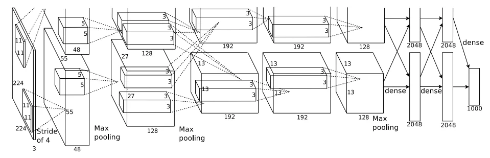
Figure 2, network architecture and two-GPU partition in Section 3.5: showing the 224×224×3 input, dimensions across five convolutional layers and three fully connected layers, within-GPU local connections for layers 2, 4, and 5 on two 3GB GTX 580 GPUs, and cross-GPU communication in layer 3 and the classifier. Original Figure 2 source. This figure is taken from the NeurIPS 2012 proceedings; copyright remains with the authors and publisher. It is reproduced here for scholarly review and educational commentary without claiming a CC BY license.

The forward layer sequence can be traced mathematically:

• Convolutional Layer 1 (Conv1): Filters the $224 \times 224 \times 3$ input image (conceptually $227 \times 227 \times 3$ with zero-padding) using 96 kernels of size $11 \times 11 \times 3$ with stride $s = 4$. Output feature map dimensions are $55 \times 55 \times 96$. Kernels are partitioned evenly across GPU 1 and GPU 2 (48 kernels per GPU). Output passes through ReLU, Local Response Normalization (LRN), and overlapping max pooling ($3 \times 3$, stride 2), downsampling spatial dimensions to $27 \times 27 \times 96$;
• Convolutional Layer 2 (Conv2): Uses 256 kernels of size $5 \times 5 \times 48$, padding 2. Critically, kernels on GPU 1 and GPU 2 connect only to the Conv1 feature maps on the same GPU. Output dimension is $27 \times 27 \times 256$. Following ReLU, LRN, and overlapping pooling, dimensions drop to $13 \times 13 \times 256$;
• Convolutional Layer 3 (Conv3): Uses 384 kernels of size $3 \times 3 \times 256$, padding 1. Here, a cross-GPU cross-bar connection occurs: kernels on both GPUs read all 256 feature maps from Conv2 across both GPUs. Output is $13 \times 13 \times 384$ (192 feature maps per GPU), followed by ReLU;
• Convolutional Layer 4 (Conv4): Uses 384 kernels of size $3 \times 3 \times 192$, padding 1. Reverts to intra-GPU local connectivity, reading only the Conv3 maps on the same chip. Output is $13 \times 13 \times 384$, followed by ReLU;
• Convolutional Layer 5 (Conv5): Uses 256 kernels of size $3 \times 3 \times 192$, padding 1, retaining intra-GPU connections. Followed by ReLU and overlapping max pooling, spatial resolution resolves to $6 \times 6 \times 256$ (128 channels per GPU);
• Dense Layers (FC6, FC7, FC8): FC6 connects all $6 \times 6 \times 256 = 9,216$ flattened features across both GPUs to 4,096 units; FC7 has 4,096 units; FC8 outputs 1,000 logits to a Softmax classifier. FC6 and FC7 utilize ReLU and Dropout.

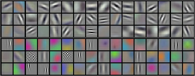
Figure 3, Section 3.5 and Section 6 of the paper (first convolutional layer feature visualization): the top 48 kernels were learned on GPU 1 and exhibit color-agnostic directional edges, while the bottom 48 kernels were learned on GPU 2 and specialize in color blobs, illustrating functional specialization from the dual-GPU split. See the original Figure 3 source. Image copyright belongs to original authors and NeurIPS; reproduced under fair scholarly commentary without CC BY claim.

Non-saturating non-linearity (ReLU)

Standard neurons with activation function $f(x) = \tanh(x)$ or $f(x) = (1 + e^{-x})^{-1}$ saturate when $|x|$ is large, causing vanishing gradients.

AlexNet adopted the Rectified Linear Unit introduced by Nair and Hinton (2010):

$$f(x) = \max(0, x)$$

For all $x > 0$, the derivative is strictly 1. Gradients propagate backward through deep compositions without exponential geometric decay. In Section 3.1 and Figure 1, the authors demonstrated that on a four-layer convolutional network on CIFAR-10, a ReLU network reached 25% training error in one-sixth the iterations required by an identical network using $\tanh$.

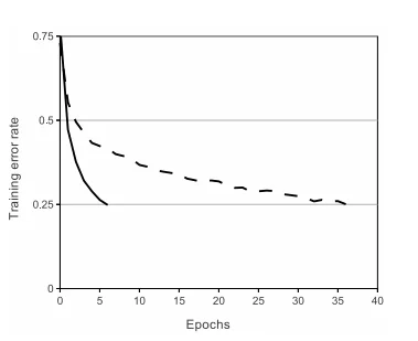
Figure 1, Section 3.1 of the paper (non-saturating nonlinearity diagnosis): solid line shows ReLU and dashed line shows tanh; reaching 25% training error with ReLU is six times faster than with tanh, demonstrating the decisive effect of non-saturating activations on gradient descent speed. See the original Figure 1 source. Image copyright belongs to original authors and NeurIPS; reproduced under fair scholarly commentary without CC BY claim.

Local Response Normalization (LRN)

Inspired by lateral inhibition in biological neural systems, Section 3.3 introduced LRN applied after ReLU in selected layers:

$$b_{x,y}^i = \frac{a_{x,y}^i}{\left(k + \alpha \sum_{j=\max(0, i-n/2)}^{\min(N-1, i+n/2)} (a_{x,y}^j)^2\right)^\beta}$$

Here, $a_{x,y}^i$ denotes the activation of kernel $i$ at spatial coordinates $(x,y)$, and $N$ is the total channel count. Hyperparameters were tuned on validation data to $k = 2$, $n = 5$, $\alpha = 1 \times 10^{-4}$, and $\beta = 0.75$.

LRN normalizes energy across neighboring feature channels, functioning as local brightness normalization. It does not subtract running means or track mini-batch statistics across instances, making it mathematically distinct from modern Batch Normalization or Layer Normalization.

Overlapping pooling

Conventional pooling arrangements set pooling window size $z \times z$ equal to stride $s$ ($s = z$). AlexNet deployed overlapping pooling in Section 3.4 with $s = 2$ and $z = 3$ ($s < z$). Compared to non-overlapping pooling ($s = 2, z = 2$), the authors observed top-1 and top-5 error reductions of 0.4% and 0.3%, noting that overlapping grids appeared slightly less susceptible to overfitting.

Data augmentation pipeline

To regularize 60 million parameters against ImageNet’s training set, Section 4.1 implemented two compute-efficient augmentation forms:

1. Random cropping and horizontal reflection: Extracting random $224 \times 224$ patches from $256 \times 256$ images alongside horizontal mirrors yields $(256 - 224 + 1)^2 \times 2 = 2,178 \approx 2,048$ potential variants. However, these spatial samples are strongly correlated and must not be misconstrued as 2,048 independent images;
2. RGB PCA color perturbation: The authors ran principal component analysis over RGB pixel values across the entire ImageNet training set. For each image, let eigenvectors be $\mathbf{p}_1, \mathbf{p}_2, \mathbf{p}_3$ with corresponding eigenvalues $\lambda_1, \lambda_2, \lambda_3$. For each training step, random Gaussian coefficients $\alpha_i \sim \mathcal{N}(0, 0.1)$ are sampled once per image, adding:

$$\Delta I_{xy} = [\mathbf{p}_1, \mathbf{p}_2, \mathbf{p}_3] [\alpha_1 \lambda_1, \alpha_2 \lambda_2, \alpha_3 \lambda_3]^T$$

This perturbation models illumination and natural color variance without distorting structural object identity.

Dropout regularization

In FC6 and FC7, Dropout sets the output of each hidden neuron to zero with probability $p = 0.5$. Dropped neurons neither participate in the forward pass nor receive gradient updates.

Every training batch effectively samples an independent sub-network architecture sharing underlying weights. Because units cannot rely on the guaranteed presence of specific co-features, they must learn self-contained, robust visual primitives. At test time, all neurons remain active, with their weights scaled by 0.5 to approximate the geometric mean of the ensemble. The authors reported that training without Dropout resulted in severe overfitting, while incorporating Dropout doubled the epochs required to reach convergence.

Optimization dynamics and learning rate schedule

The network was trained using stochastic gradient descent (SGD) with batch size 128, momentum 0.9, and weight decay 0.0005. The parameter update equation follows:

$$v_{t+1} = 0.9 \cdot v_t - 0.0005 \cdot \epsilon \cdot w_t - \epsilon \cdot \left\langle \left. \frac{\partial L}{\partial w} \right|_{w_t} \right\rangle_{D_i}$$ $$w_{t+1} = w_t + v_{t+1}$$

where $i$ is iteration, $v$ is momentum velocity, $\epsilon$ is learning rate, and $\langle \cdot \rangle_{D_i}$ denotes the average loss gradient over mini-batch $D_i$. In Section 5, the authors noted that 0.0005 weight decay was not merely a regularizer; it measurably reduced training error in this configuration.

The initial learning rate was set to $\epsilon = 0.01$. Training followed a manual heuristic: whenever validation error plateaued, the learning rate was divided by 10. Over roughly 90 epochs spanning 5 to 6 days across two 3GB GTX 580 GPUs, the learning rate was dropped three times.

How to read the evidence

Reading AlexNet’s empirical results requires separating module-level diagnostic checks from whole-system competition metrics, ensuring individual performance deltas are not confounded.

Experimental environment and dimensions

Experiments spanned two primary benchmarks:

• ILSVRC-2010: Included 1.2M training images, 50,000 validation images, and 150,000 test images with publicly released test ground truth. Evaluated using top-1 and top-5 error rates;
• ILSVRC-2012: Competition setting with withheld test labels, evaluated through official server submissions.

Baselines encompassed leading handcrafted feature systems: NEC’s Sparse Coding and the University of Amsterdam’s dense SIFT with Fisher Vectors.

Component-level diagnostics

Sections 3 and 4 report isolated component ablations:

1. ReLU convergence speed (Section 3.1; Figure 1): On a four-layer CIFAR-10 CNN, ReLU reached 25% training error six times faster than $\tanh$. Boundary: This is an optimization speed benchmark on a small network, not a direct ImageNet accuracy ablation;
2. Dual-GPU topology gains (Section 3.2): Compared to a single-GPU network with half the kernels per layer, the dual-GPU design reduced top-1 and top-5 errors by 1.7% and 1.2%. Boundary: Footnote 4 acknowledges that the single-GPU model retained full-sized final convolutional and dense layers, slightly biasing the comparison;
3. Local Response Normalization (Section 3.3): On a four-layer network, LRN reduced top-1 and top-5 error by 1.4% and 1.2%;
4. Overlapping pooling (Section 3.4): $s=2, z=3$ pooling reduced top-1 and top-5 error by 0.4% and 0.3% over $s=2, z=2$ pooling;
5. PCA color augmentation (Section 4.1): Reported to reduce top-1 error by over 1.0 percentage point;
6. Dropout against overfitting (Section 4.2): Omitting Dropout caused substantial overfitting, while its inclusion roughly doubled the iterations required to reach convergence.

Benchmark comparisons (Table 1 and Table 2)

On the ILSVRC-2010 test set (Table 1):

• Sparse Coding baseline: 47.1% top-1, 28.2% top-5;
• Fisher Vector baseline (SIFT + FVs): 45.7% top-1, 25.7% top-5;
• AlexNet (Single CNN): Achieved 37.5% top-1 and 17.0% top-5.

In the ILSVRC-2012 competition (Table 2 and Section 6):

• Best competing traditional vision entry: 26.2% top-5;
• AlexNet single model: 18.2% top-5;
• AlexNet 5-model ensemble: 16.4% top-5;
• AlexNet 6-model ensemble (with pre-training data): 15.3% top-5.

This decisive margin established the dominance of deep convolutional networks. However, the result represents the cumulative outcome of the entire system recipe—ReLU, multi-GPU splitting, data augmentation, Dropout, and SGD scheduling—and cannot be credited to depth alone.

Evidence map

To clarify the empirical status of the paper’s claims, its findings are decomposed into four distinct evidential layers:

Direct paper evidence

1. ReLU optimization acceleration: Section 3.1 and Figure 1 prove that on a four-layer CIFAR-10 CNN, substituting $\tanh$ with ReLU reduced training iterations to 25% error by a factor of six;
2. Multi-GPU error reduction: Section 3.2 establishes that the two-GPU partition reduced top-1 and top-5 error by 1.7% and 1.2% relative to a capacity-constrained single-GPU model;
3. Marginal gains from LRN and overlapping pooling: Sections 3.3 and 3.4 report error reductions of 1.4%/1.2% for LRN and 0.4%/0.3% for overlapping pooling;
4. Regularization efficacy: Section 4.1 demonstrates >1% top-1 gain from PCA color augmentation; Section 4.2 demonstrates that Dropout prevented catastrophic overfitting in the 60M-parameter dense layers;
5. Benchmark margin: Table 1 establishes a 37.5%/17.0% error rate on ILSVRC-2010, surpassing the best Fisher Vector baseline (45.7%/25.7%).

Author causal claim

1. ReLU as an absolute necessity for scale: The authors argue that without ReLU, gradient vanishing would have rendered training an eight-layer CNN impossible within practical timeframes on 2012 hardware;
2. Dual-GPU topology as the optimal capacity-bandwidth compromise: The authors claim that restricting communication in Conv2, Conv4, and Conv5 while allowing cross-talk in Conv3 and dense layers maximized feature representation given GTX 580 memory limits;
3. Dropout as implicit ensemble averaging: The authors frame Dropout as an approximation to training an exponential ensemble of sub-networks with shared weights;
4. Weight decay aiding optimization: The authors hypothesize that in this specific SGD setup, 0.0005 weight decay actively assisted optimization rather than acting solely as an L2 penalty.

Unsupported claims

1. Lack of full factorial ablation: Component checks were executed on disparate smaller networks or separate subsets. The paper does not prove that removing LRN or overlapping pooling from the complete, Dropout-regularized AlexNet causes statistically significant degradation;
2. No comparison with data parallelism: Constrained by early custom CUDA routines, the authors did not provide a standardized throughput comparison against full data parallelism;
3. LRN as a universal normalization: The paper lacks comparison against modern normalization techniques (BatchNorm, LayerNorm), nor does it demonstrate stability in significantly deeper networks;
4. Selection bias from manual validation tuning: Learning rate schedule drops and LRN constants were tuned interactively on the validation set without multi-seed confidence intervals.

Bloss0m engineering synthesis

1. System recipe over isolated tricks: AlexNet’s breakthrough was fundamentally hardware-driven systems engineering. Over-emphasizing 11×11 kernels while ignoring VRAM constraints and data augmentation misinterprets its technical contribution;
2. Separating historical artifacts from timeless principles: Dual-GPU channel grouping and LRN were compromises for 2012 hardware. Modern practitioners should replace them with Distributed Data Parallel (DDP) and BatchNorm/LayerNorm;
3. Decoupled experimental hypotheses: In vision benchmarks, engineers must strictly isolate representational capacity (architecture), optimization convergence (activation and optimizer), and generalization bounds (augmentation and regularization).

Artifacts and reproducibility

This analysis is grounded in the formal paper published at NeurIPS 2012. Evaluating its reproducibility requires distinguishing historical code repositories from modern framework implementations.

As of 2026-08-09, the author’s original cuda-convnet Google Code repository is an unmaintained historical archive that relies on obsolete hardware-specific assembly and legacy CUDA driver APIs; it cannot function as a runnable out-of-the-box modern artifact. The accessible and widely validated reference artifact is the BVLC Caffe AlexNet model definition, which provides verified prototxt definitions and pre-trained weights, categorizing it as a usable partial artifact.

Engineers should delineate three distinct reproduction levels:

1. Functional reconstruction: Implementing Figure 2’s equivalent layer sequence in PyTorch or JAX, matching layer dimensions and tensor shapes. This level is 100% reproducible today;
2. Protocol reconstruction: Matching $224 \times 224$ crops, reflections, PCA color jitter, Dropout 0.5, SGD momentum 0.9, weight decay 0.0005, and validation-guided step drops. This protocol is fully reproducible;
3. Numerical reconstruction: Attempting to reproduce Table 1 (37.5%/17.0%) or Table 2 (15.3%) errors to exact bit-level precision. Because ILSVRC competition test labels were withheld, floating-point GPU operations are non-deterministic, and the original learning rate schedule involved manual human intervention, exact numerical replication is objectively unavailable.

Independent rerun scope: All experimental metrics cited herein originate from the authors’ published reports. This deep dive did not re-train AlexNet from scratch across ImageNet, but conducted an engineering audit of the paper’s mathematical formulations, empirical claims, and public reference models.

Bloss0m engineering judgment and when not to use it

Drawing from production machine learning engineering practices, this section outlines specific adoption boundaries for AlexNet’s techniques:

When to adopt AlexNet’s methodology

1. Establishing baseline CNN pipelines: When building custom small-scale vision models for edge hardware, AlexNet’s “Augmentation + ReLU + Momentum SGD + Step Decay” provides a dependable minimal baseline;
2. Decoupling data loading from compute throughput: Adopting the pipeline design of overlapping CPU data decoding and augmentation while the GPU processes preceding batches prevents GPU compute starvation;
3. Granular regularization ablations: Separating geometric transformations, color perturbations, and Dropout to evaluate their marginal generalization value independently.

When not to use it

1. Do not use Local Response Normalization (LRN): LRN is computationally inefficient and superseded by Batch Normalization and Layer Normalization. Retaining LRN adds kernel latency without modern statistical benefits;
2. Do not replicate dual-GPU channel grouping: Figure 2’s local connectivity in Conv2, Conv4, and Conv5 was a workaround for 3GB VRAM limits. Modern GPUs easily hold the model; multi-device training should utilize standard Distributed Data Parallel (DDP) or Tensor Parallelism;
3. Do not deploy 10-crop inference in real-time serving: Running 10 forward passes increases serving latency and inference costs tenfold. Modern backbones with single-crop evaluation yield far superior accuracy at a fraction of the cost;
4. Do not use manual step decay: Relying on manual human observation of validation loss is error-prone. Modern training should deploy automated Cosine Annealing with Warmup or automated plateau schedulers.

For an examination of the degradation problem in deeper plain networks and how residual shortcuts resolve it, continue to the companion deep dive: ResNet Deep Dive: The Essence of Deep Residual Learning.

Three things to remember

1. Technical idea: AlexNet’s historical advance was not merely adding depth, but unifying non-saturating activations (ReLU), multi-GPU memory layout, empirical distribution expansion, and implicit ensembling (Dropout) into an end-to-end trainable system.
2. Core evidence: ReLU accelerated training convergence sixfold on small CNNs, PCA color augmentation added over 1% top-1 accuracy, and the complete system achieved 37.5%/17.0% on ILSVRC-2010, outperforming traditional Fisher Vector baselines by over 8 percentage points.
3. Engineering boundary: The paper presents single-factor diagnostics rather than a factorial ablation matrix; LRN, dual-GPU kernel splitting, and 10-crop inference were specific hardware workarounds that should be replaced with BatchNorm, DDP, and single-crop inference in modern pipelines.

Primary sources

• Full AlexNet Paper PDF (NeurIPS 2012): Figure 1–3, Sections 3–6, Table 1–2.
• BVLC Caffe AlexNet Model Repository: Community-validated reference model definition (prototxt and weights).
• AlexNet Part 1: Reading Why It Changed ImageNet Through Evidence: Part 1 of this series, focusing on competition benchmarks, problem formulation, and macro-architecture.
• ResNet Deep Dive: The Essence of Deep Residual Learning: Architectural evolution addressing deep network degradation via residual shortcut connections.