AlexNet Part 1: Reading the Evidence Behind an ImageNet Turning Point

The paper in 90 seconds

• Problem: In 2012, scaling deep convolutional neural networks (CNNs) to high-resolution datasets containing millions of images was blocked by three simultaneous engineering bottlenecks: severe gradient optimization difficulties under saturating activations, rigid GPU memory ceilings (a mere 3GB per card), and disastrous overfitting on high-capacity models lacking modern regularization.
• Core insight: AlexNet’s breakthrough was not an isolated “make the network deeper” mantra, but the synthesis of convolutional spatial inductive bias, non-saturating ReLU activations, cross-GPU memory partitioning, overlapping pooling, and aggressive regularization (Dropout and multi-faceted data augmentation) into the first practically trainable, end-to-end deep vision system.
• Strongest evidence: On the ILSVRC-2010 test set, AlexNet achieved 37.5% top-1 and 17.0% top-5 error, decisively beating the best contemporary SIFT + Fisher Vector baseline (45.7% / 25.7%); in the ILSVRC-2012 competition, its 7-CNN ensemble secured victory with 15.3% top-5 error against 26.2% for the second-place entry (Section 6, Table 1, Table 2).
• Main boundary: Local Response Normalization (LRN), custom cross-GPU channel splitting tailored to dual 3GB GTX 580 cards, and large 11×11 stride-4 first-layer filters were hardware-era compromises, not timeless architectural recommendations for modern accelerator systems or broad visual domains.

The 2012 NeurIPS paper ImageNet Classification with Deep Convolutional Neural Networks is universally cited as the catalyst that ignited the modern deep learning revolution. Yet in retrospective retellings, this achievement is frequently reduced to a slogan: “deep networks simply outperformed handcrafted features on ImageNet.” That shorthand conceals the genuine engineering triumph: in an era dominated by hand-tuned feature pipelines and shallow classifiers, how did the authors coax a 60-million parameter neural network to converge reliably under acute memory and compute constraints? This article serves as Part 1 of our AlexNet deep dive, addressing the problem formulation, evaluation protocol, historical empirical findings, and evidence boundaries. The detailed layer dimensions, data augmentation, Dropout dynamics, and trainability mechanics are unpacked in Part 2: AlexNet Architecture and Training Recipe.

What to know first

1. ImageNet and the ILSVRC benchmark: Section 2 draws an essential distinction between the full ImageNet collection (over 15 million labelled high-resolution images spanning approximately 22,000 categories) and the annual ILSVRC subset (ImageNet Large-Scale Visual Recognition Challenge). All central experiments in the paper evaluate the 1,000-category ILSVRC benchmark, comprising roughly 1.2 million training images, 50,000 validation images, and 150,000 test images with fixed labels (Section 2). Because image resolutions vary widely, inputs must undergo standardized geometric preprocessing before entering the network.
2. Classification metric: Top-1 vs. Top-5 error rates: The evaluation uses classification error rates. An inference instance incurs a Top-1 error if the highest-probability category prediction does not match the ground-truth label; it incurs a Top-5 error only if the ground truth is entirely absent from the model’s five highest-probability predictions. Top-5 error was adopted because ImageNet contains fine-grained categories and multi-object scenes where multiple labels could be plausible, providing a robust evaluation metric that attenuates single-label ambiguity.
3. Why previous approaches were insufficient (traditional method bottlenecks): Before AlexNet, computer vision was dominated by multi-stage pipelines: hand-engineered local feature descriptors (such as SIFT, HOG, or LBP), followed by vector quantization encodings (such as Bag-of-Visual-Words, Sparse Coding, or Fisher Vectors), and finally classified by linear or kernel Support Vector Machines (SVMs). Why did these traditional methods hit a wall?
   • Representation capacity ceiling: Handcrafted features impose rigid human heuristics. While effective on small benchmarks (like Caltech-101 or NORB), shallow feature pipelines lack the representational bandwidth required to absorb the massive intra-class variance, scale changes, and complex lighting in 1.2 million images.
   • The vanishing gradient optimization bottleneck: Prior attempts to train deep networks predominantly relied on saturating activation functions such as the hyperbolic tangent $f(x) = \tanh(x)$ or the logistic sigmoid $f(x) = (1 + e^{-x})^{-1}$. Because their derivatives approach zero when the input magnitude is even moderately large, backpropagated error gradients decayed exponentially through depth, rendering gradient-based optimization intolerably slow or entirely stuck.
   • The 2012 hardware memory wall: A flagship consumer GPU in 2012, the NVIDIA GeForce GTX 580, offered only 3GB of VRAM. A single card could not physically store 60 million parameters alongside the intermediate activation tensors and gradient buffers required during backpropagation on high-resolution images.

Core intuition

Under the traditional paradigm, the decision pipeline was decoupled: human experts designed static filter banks, image descriptors were aggregated into fixed high-dimensional histograms, and an SVM learned a separating hyperplane. If the handcrafted descriptor failed to capture an essential subtle structural cue, the classifier had no mechanism to rectify that upstream perceptual defect.

AlexNet replaces this with end-to-end representation learning:

1. Structural exploitation of visual inductive bias: Flattening a 224×224×3 RGB patch into a 150,000-dimensional vector for a standard Multi-Layer Perceptron (MLP) would produce an explosion of parameters, erase spatial topography, and severely overfit. Convolution enforces weight sharing and local receptive fields, directly leveraging two universal statistical invariants of natural imagery: stationarity (features are invariant to spatial translation) and pixel locality (neighboring pixels exhibit strong mutual correlation).
2. Non-saturating activation dynamics: Swapping saturating functions for the piecewise linear Rectified Linear Unit, $f(x) = \max(0, x)$, ensures that the gradient remains constant ($1$) for any positive pre-activation. This prevents gradient vanishing across successive layers, fundamentally unlocking deep gradient-based learning.
3. Hardware memory co-design: Rather than treating GPU memory as an invisible backend concern, the authors treated hardware boundaries as an explicit architectural design constraint. Splitting convolutional kernels across two GPUs and permitting cross-GPU communication only at specific bottleneck layers (Layer 3 and the fully connected layers) balanced representational capacity against interconnect bandwidth limitations.

Walk one example through the method

1. Input: A raw arbitrary-resolution RGB image is resized with its shorter edge scaled to 256 pixels, followed by a central 256×256 crop. The training-set mean RGB pixel value is subtracted. At test time, ten 224×224 crops are extracted: four corners plus one center crop, along with their horizontal mirror reflections.
2. Intermediate representation:
   • Layer 1 (Conv1): 96 kernels of size 11×11×3 with stride 4 process the 224×224×3 patch, producing a 55×55×96 feature map (48 channels per GPU). Features represent low-level oriented edges and color blobs. This is followed by ReLU, Local Response Normalization (LRN), and 3×3 overlapping max pooling with stride 2, reducing spatial resolution to 27×27×96.
   • Layer 2 (Conv2): 256 kernels of size 5×5 (128 per GPU) operate locally within each GPU, followed by ReLU, LRN, and overlapping pooling, yielding a 13×13×256 representation.
   • Layers 3–5 (Conv3–Conv5): Layer 3 uses 384 kernels of size 3×3, connecting across the feature maps of both GPUs to integrate composite textures. Layer 4 (384 kernels, 3×3) and Layer 5 (256 kernels, 3×3) revert to within-GPU local connections. A final overlapping max pooling stage reduces the volume to 6×6×256 (128 channels per GPU).
   • Fully connected layers (FC6–FC7): The 6×6×256 tensor is flattened into a 9,216-dimensional vector and fed into FC6 (4,096 units, fully connected across both GPUs), followed by FC7 (4,096 units). Both employ ReLU and 50% Dropout during training.
3. Decision or transformation: FC7 projects into FC8, generating 1,000 unnormalized logits $z_i$, which pass through a 1,000-way softmax function: $p_i = \frac{e^{z_i}}{\sum_{j=1}^{1000} e^{z_j}}$ At inference, the softmax probability distributions from all ten crops are averaged to produce the final robust class posterior.
4. Output: A ranked list of the top-5 predicted category labels with associated probabilities. If the ground-truth category matches the top-ranked prediction, both Top-1 and Top-5 errors are zero; if it falls within the top five candidates, Top-1 is an error but Top-5 is counted as a success.
5. Likely failure point: If early convolutional layers fail to capture discriminatory textures due to severe motion blur, low contrast, or extreme perspective distortion, deeper layers cannot reconstruct the missing geometric evidence. Furthermore, if a small target object is located near the perimeter of the frame, single-crop evaluation may miss it entirely, explaining the measurable ~1.2% error reduction provided by ten-crop averaging.

Technical mechanism

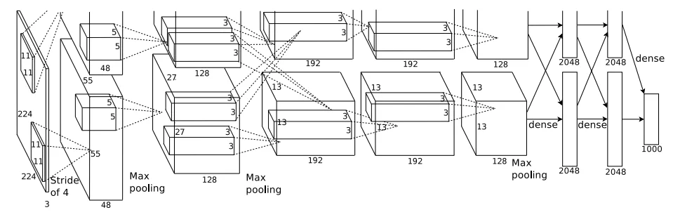
Figure 2, the network architecture in Section 3.5: it makes the split, local connections, and layer-by-layer spatial reduction concrete. See the original Figure 2 source. This figure comes from the NeurIPS 2012 proceedings; copyright remains with the authors/publisher, and this article preserves the source for scholarly commentary without claiming a CC BY license.

1. ReLU Non-saturating Activation (Section 3.1): Defined as $f(x) = \max(0, x)$. In Figure 1, the authors compare a four-layer convolutional network on CIFAR-10 equipped with ReLUs against an identical network equipped with $\tanh$ neurons. The ReLU network reached a 25% training error threshold six times faster than the $\tanh$ equivalent.
2. Multi-GPU Parallelization Scheme (Section 3.2): Driven by the 3GB VRAM ceiling of NVIDIA GTX 580 GPUs, the network partitions its kernels equally across two cards. GPUs communicate directly via peer-to-peer DMA over the PCIe bus. Layer 2 reads only from Layer 1 on the same GPU; Layer 3 connects to all Layer 2 feature maps across both GPUs; Layers 4 and 5 connect only within the same GPU; FC layers connect across all units on both GPUs. The authors report that this two-GPU split reduced top-1 error by 1.7% and top-5 error by 1.2% compared to an equal-capacity single-GPU design (with noted minor parameter mismatches).
3. Local Response Normalization (LRN, Section 3.3): Expressed as: $b_{x,y}^i = \frac{a_{x,y}^i}{\left(k + \alpha \sum_{j=\max(0, i-n/2)}^{\min(N-1, i+n/2)} (a_{x,y}^j)^2\right)^\beta}$ with hyperparameters $k=2, n=5, \alpha=10^{-4}, \beta=0.75$. It applies lateral inhibition across $n$ adjacent kernel channels at identical spatial coordinates, curbing runaway activations. The authors report that LRN reduced top-1 error by 1.4% and top-5 error by 1.2% on a four-layer CNN. Though later superseded by Batch Normalization, LRN was a pivotal early technique for stabilising deep network activations.
4. Overlapping Pooling (Section 3.4): Instead of standard disjoint pooling where stride $s$ equals kernel size $z$, AlexNet uses $z=3, s=2$. The authors report a 0.4% reduction in top-1 error and 0.3% in top-5 error, noting that overlapping pooling rendered the network slightly less susceptible to overfitting.
5. Full Network Dimensions and Parameter Distribution (Section 3.5): With 8 learned layers (5 convolutional, 3 fully connected), the network comprises approximately 60 million parameters and 650,000 neurons. Notably, FC6 alone ($6 \times 6 \times 256 \times 4096$) consumes roughly 37.7 million weights—over 60% of the entire model’s parameters. This stark architectural asymmetry concentrated parameter memory in the classifier head while concentrating FLOPs in the early convolutional layers.

How to read the evidence

1. Experimental setup and baseline controls:
   • Datasets: ILSVRC-2010 (1,000 classes, 1.2M training images, 50,000 validation images, 150,000 test images with ground truth); ILSVRC-2012 (test labels withheld for official server evaluation).
   • Baselines: State-of-the-art non-deep-learning entries, including Sparse Coding (Lin et al., 2011) and SIFT + Fisher Vectors (Sánchez & Perronnin, 2011).
   • Compute: Two NVIDIA GeForce GTX 580 3GB GPUs, trained using stochastic gradient descent with momentum 0.9 and weight decay 0.0005 over roughly 90 epochs, requiring 5 to 6 days.
   • Metrics: Top-1 error and Top-5 error rates.
2. ILSVRC-2010 benchmark results (Table 1): Evaluating the shared 2010 test set:
   • Sparse Coding: 47.1% top-1, 28.2% top-5 error
   • SIFT + Fisher Vectors: 45.7% top-1, 25.7% top-5 error
   • AlexNet (CNN): 37.5% top-1, 17.0% top-5 error AlexNet reduced top-1 error by 8.2 absolute percentage points and top-5 error by 8.7 absolute percentage points (a ~34% relative drop) versus the best prior method. All Table 1 numbers are test errors on fixed labels.
3. ILSVRC-2012 competition results (Table 2): Table 2 documents the 2012 competition entries:
   • Single AlexNet model: 18.2% top-5 (validation)
   • Ensemble of 5 similar CNNs: 16.4% top-5 (validation), 16.4% top-5 (test)
   • Single CNN pre-trained on ImageNet Fall 2011 (15M images, 22k classes) and fine-tuned: 16.6% top-5 (validation)
   • Ensemble of 7 CNNs (combining pre-trained and standard models): 15.3% top-5 error (test)
   • Runner-up entry (non-CNN ensemble): 26.2% top-5 error The margin of victory was an astonishing 10.9 absolute percentage points. Crucially, the 17.0% of Table 1 and the 15.3% of Table 2 represent distinct datasets and evaluation protocols (the former being a single model on 2010 test data, the latter a 7-model ensemble submitted to the 2012 competition server); they must not be conflated.

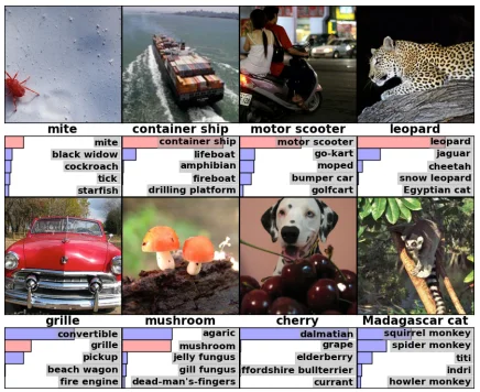
Figure 4, Section 6 of the paper (qualitative evaluations): eight ImageNet test images with the top-5 predicted labels from the model, illustrating predictions under varied object poses, occlusions, and multi-object scenes. See the original Figure 4 source. Image copyright belongs to the original authors and NeurIPS; reproduced under fair scholarly commentary without CC BY claim.

4. Diagnostic and informal ablation analysis:
   • Figure 1 provides optimization diagnostic evidence on CIFAR-10, demonstrating a 6x speedup to 25% training error for ReLU over tanh, but does not measure final ImageNet generalization.
   • The depth ablation claim: In Section 1, the authors state that removing any single convolutional layer degraded top-1 performance by roughly 2%. While revealing design sensitivity, this informal observation lacked controlled depth-versus-parameter factorial sweeps and cannot be cited as causal proof that depth alone guarantees accuracy.
   • Lack of statistical intervals: Neither Table 1 nor Table 2 reports random seed variation, confidence intervals, or per-image inference latency.

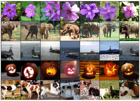
Figure 5, Section 6 of the paper (qualitative evaluations): the first column contains test images, while the remaining columns show training images with the smallest Euclidean distance in the 4,096-dimensional hidden layer feature space, demonstrating semantic representation rather than pixel-level memorization. See the original Figure 5 source. Image copyright belongs to the original authors and NeurIPS; reproduced under fair scholarly commentary without CC BY claim.

Evidence map

• Direct paper evidence (paper directly supports):
  • Table 1 demonstrates that AlexNet achieved 37.5% top-1 and 17.0% top-5 error on the ILSVRC-2010 test set, strictly outperforming SIFT+FV (45.7% / 25.7%) under an identical evaluation protocol.
  • Table 2 establishes that AlexNet’s 7-CNN ensemble achieved 15.3% top-5 error on the ILSVRC-2012 blind test set, beating the non-deep-learning runner-up (26.2%).
  • Figure 1 documents that a four-layer CNN with ReLU reached 25% training error six times faster than with tanh on CIFAR-10.
  • Sections 3.2–3.4 report author-measured local ablations: LRN yielded ~1.2% top-5 error reduction, overlapping pooling yielded ~0.3% top-5 reduction, and the two-GPU scheme yielded ~1.2% top-5 reduction.
• Author causal claims (author claims):
  • The authors assert that depth is essential, citing an approximate 2% drop in performance whenever any single convolutional layer was removed (Section 1).
  • The authors attribute their breakthrough to the triad of massive labeled data, optimized GPU parallel execution, and deep non-saturating CNN architecture.
  • The authors claim that CNN weight sharing and local connectivity supply mostly correct inductive biases for natural imagery.
• Unsupported claims (evidence boundary):
  • The paper does not prove that depth alone caused the performance leap; there is no controlled comparison holding parameter count, width, and training compute constant.
  • The paper does not test cross-domain transfer, few-shot generalization, adversarial robustness, or open-world recognition.
  • The paper does not evaluate probability calibration; a high Top-5 score does not prevent confident erroneous predictions on out-of-distribution inputs.
  • The paper does not prove that LRN or custom two-GPU tensor splits represent optimal representation components; subsequent research demonstrated that LRN is redundant under Batch Normalization, and manual tensor splits are superseded by modern data parallelism.
• Bloss0m engineering synthesis:
  • AlexNet must be treated as an integrated systems engineering recipe (data volume + GPU hardware optimization + non-saturating activation + structural regularization) rather than an isolated deep network topology.
  • Four-dimension transfer checklist:
    1. Data denominator: verify whether the target task is closed-set 1,000-class classification, or whether it exhibits long tails, open sets, or multi-label requirements that cannot lean on ILSVRC evidence.
    2. Metric alignment: distinguish single-crop from ten-crop evaluation; never use offline ten-crop accuracy to estimate low-latency production throughput.
    3. Baseline parity: benchmark modern candidates against contemporary lightweight backbones (e.g. ConvNeXt, MobileNetV4, ViT) rather than re-litigating 2012 SIFT baselines.
    4. Hardware execution model: rely on modern PyTorch DDP / FSDP data parallelism rather than manual layer-specific cross-GPU routing.

Artifacts and reproducibility

• As of August 9, 2026, the original cuda-convnet Google Code repository referenced in the paper’s footnote is archived as a read-only historical repository. It lacks compatibility with modern GPU microarchitectures and current CUDA toolchains, and cannot be treated as a turnkey modern reproduction artifact.
• The publicly accessible BVLC Caffe AlexNet model definition is a later community implementation that consolidates channels for single-GPU execution. It provides model definitions and weights, but does not include the original twin-GTX 580 custom CUDA kernels, memory layouts, or raw training pipeline.
• Modern frameworks (e.g. torchvision.models.alexnet) implement unified-channel variants of AlexNet, typically omitting LRN or altering stride/padding details, yielding ~56.5% top-1 accuracy (~43.5% single-crop error) on standard ImageNet.
• ImageNet (ILSVRC) requires formal researcher registration and institutional approval via official channels; ground-truth labels for the 2012 competition test set were never made publicly downloadable.
• The experimental values in this article represent author-reported results from the NeurIPS 2012 paper; the full benchmark was not rerun for this reading. Any modern reproduction should fix an authorized ImageNet split, specify single-crop or ten-crop protocols, and label the outcome an “AlexNet-like reproduction” rather than claiming replication of the 2012 competition submission environment.

Bloss0m engineering judgment and when not to use it

• Durable engineering principles:
  1. Hardware-software co-design: when model scale collides with hardware limits, treat memory and bandwidth as explicit architectural priors, designing network layouts that match hardware characteristics.
  2. Protect gradient flow: non-saturating activation functions are the foundational prerequisite for deep optimization, a principle inherited by modern GELU and Swish activations.
  3. Balance capacity with data scale: increasing model capacity without commensurate labeled data and regularization guarantees catastrophic overfitting.
• When NOT to use AlexNet in modern engineering:
  • Do NOT deploy AlexNet as a production vision backbone: modern architectures (e.g., ConvNeXt, MobileNetV4, EfficientNet, ResNet) achieve drastically higher accuracy (>80% vs ~62.5% top-1) with a fraction of the parameter count and computational footprint.
  • Do NOT implement LRN: Local Response Normalization is computationally awkward and lacks cross-batch distributional stabilization; it has been comprehensively superseded by Batch Normalization, Layer Normalization, and RMSNorm.
  • Do NOT write custom layer-specific cross-GPU splits: modern distributed training relies on framework-level abstractions (PyTorch DDP, FSDP, DeepSpeed) and optimized communication libraries (NCCL) rather than hand-crafted tensor routing.
  • Do NOT rely on Top-5 error for safety-critical systems: in medical imaging, autonomous vehicles, or industrial inspection, incorrect classifications within the top five are unacceptable, and decisions require rigorously calibrated probabilities or rejection thresholds.

Three things to remember

1. Technical idea: AlexNet’s breakthrough was building the first practically trainable million-scale vision system; convolutional inductive bias, non-saturating ReLU activations, cross-GPU memory partitioning, and Dropout jointly conquered deep optimization and overfitting.
2. Core evidence: On the shared ILSVRC-2010 test set, AlexNet achieved 37.5% top-1 and 17.0% top-5 error, improving upon the state-of-the-art SIFT+Fisher Vector baseline by 8.2 and 8.7 absolute percentage points; its 2012 competition ensemble achieved 15.3% top-5 error, defeating the non-deep-learning runner-up by 10.9 points.
3. Engineering boundary: The two-GPU communication topology, LRN, and massive 11×11 kernels were hardware-era compromises for 3GB VRAM. Modern engineering should inherit the systems lesson—co-designing compute, data, and trainability—rather than copying obsolete architectural hyperparameters.

Primary sources

• Krizhevsky, Sutskever, and Hinton, full NeurIPS 2012 paper: Section 1–2, Figure 1–2, Table 1–2.
• BVLC Caffe AlexNet model definition: scope of accessible later artifacts.
• Series navigation: This article is Part 1 of the two-part AlexNet series, focusing on problem setup, evaluation protocol, and historical empirical evidence. For layer-by-layer architectural dimensions, trainability mechanisms, regularization, and the data pipeline, see Part 2: AlexNet Architecture and Training Recipe.