When Is Complex Chunking Worth It? Reading a Multi-Objective Chunking Evaluation

The paper in 90 seconds

• Problem: Long documents may exceed an embedding model’s usable input length. Splitting them changes the granularity of searchable content and can also increase vector count, indexing time, query work, and memory. A limitation of prior approaches is that chunking comparisons often focus on retrieval scores without reporting system costs alongside them.
• Core insight: The authors place eight chunking strategies in one multi-objective evaluation across two corpora, three embedding models, and multiple corpus sizes. They measure retrieval effectiveness alongside indexing and serving costs.
• Strongest evidence: The significant-win matrices in Figure 1 change between NDCG@10 and Recall@100; the scores in Table 2 also shift with model, data, and scale; and Figure 2 shows that similar retrieval quality can come with different throughput and memory.
• Main boundary: This is a dense-retrieval evaluation, not a test of generated answers or a complete RAG system. Some expensive methods were not run at the largest corpus sizes, and runtime results describe a specific implementation and hardware setup.

Reading verdict: The paper does not prove that simple chunking is always best. It finds that expensive methods rarely beat simple ones consistently. Choose a strategy according to the service stage, target metric, and indexing budget; use the results to design a local comparison rather than as a production ranking.

Source version and paper status

This reading follows arXiv v1, dated August 17, 2026. The authors are Laura Caspari, Kanishka Ghosh Dastidar, Michael Dinzinger, Jelena Mitrović, and Michael Granitzer. A footnote in v1 says the paper was accepted to ACM CIKM 2026. As of September 26, 2026, the conference is still scheduled for November 7–11, so this reading describes the paper as accepted rather than implying that its proceedings have already appeared.

The paper broadens chunking from “which split maximizes a retrieval score?” to a systems choice: the representation of each searchable unit affects retrieval quality as well as index size, construction speed, query speed, and peak memory. Its central finding is that computationally expensive strategies rarely beat simpler ones consistently. Results vary with the embedding model, dataset, corpus size, and target metric.

Core intuition: chunking changes the search units and the cost

Dense retrieval embeds a query and searchable content, then finds candidates by vector similarity. A single vector for a long document may truncate text beyond the model’s usable length or blend distinct topics. Splitting the document makes local passages independently searchable, but may create more vectors per document. More vectors can enlarge the index; generating context for every chunk can also extend construction time.

Imagine a long manual with sections on account recovery and two-factor authentication. A fixed token window might split a heading from its steps. Sentence chunking avoids breaking in the middle of a sentence but does not necessarily know which section the sentence belongs to. Adding a document title to each chunk supplies a topic cue; adding a document summary brings in document-level context but requires summary generation. Contextual chunking goes further and generates a local explanation for each chunk based on the full document. These operations change the content and count of the indexed units, not merely the delimiter used to divide a fixed string.

The eight strategies in the paper change different parts of this process. They do not form a simple ladder from “basic” to “intelligent.”

Method	Operation in the paper	Extra work and what to watch
Token	Splits into fixed token windows, optionally with overlap	Direct and usually fast to index; boundaries can cut through sentences.
Sentence	Adjusts token windows so chunks end at sentence boundaries	Preserves complete sentences, but variable sentence length affects throughput; a sentence boundary is not necessarily a semantic or section boundary.
Late	Encodes a full document, chunks unpooled token embeddings, then aggregates them into chunk vectors	Uses document-wide encoding context; intermediate representations can raise indexing memory.
Enriched (Title)	Prepends the document title to each chunk	Requires no extra LLM generation; value depends on whether titles provide useful cues.
Enriched (Summary)	Prepends a document-level summary to each chunk	Summary generation adds construction work while giving each local chunk a document-level overview.
Contextual	Generates context for each chunk from the full document and prepends it	Requires generation per chunk, so throughput and cost depend on the generation service.
Summary	Uses a generated document summary as the document’s retrieval representation	One representation per document makes the query index smaller; local details may be harder to retrieve.
Semantic	Groups sentences using sentence-embedding similarity to decide chunk boundaries	Boundaries depend on the embedding model and similarity threshold; sentence encoding adds work.

For Token, Sentence, Late, both Enriched methods, and Contextual, the experiment uses 512-token chunks with 25-token overlap before adding optional metadata or generated context. Semantic chunking encodes sentences with the retrieval embedder and starts a new chunk when similarity falls below the 95th-percentile threshold. Summary and Contextual use a locally run, 8-bit-quantized Qwen3-Next-80B-A3B-Instruct model; generated outputs are reused across embedding models where applicable. These are the authors’ comparison settings, not recommended optimal parameters for every product.

Walk one query through the evaluation

“How do I reset two-factor authentication in this manual?” is a Bloss0m explanatory example to make the protocol concrete; it is not a query reported as tested by the authors.

1. Input: Fix a document set, queries, and relevance judgments. Each chunking strategy sees the same input so their retrieval scores can be compared.
2. Create search units: The eight chunkers split or enrich the documents in different ways. Token uses fixed windows; Enriched (Title) adds document titles; Summary and Contextual first generate summaries or chunk context; Semantic uses sentence-vector similarity to select boundaries.
3. Encode and index: A selected embedding model encodes each strategy’s output into vectors stored in FAISS. Strategies can create different numbers of vectors, changing both indexing work and the items compared for a query.
4. Retrieve and score: The system retrieves high-ranked chunks and maps chunk-level scores back to documents. NDCG@10 measures top-ten ordering; Recall@100 asks whether relevant documents appear among the first hundred candidates.
5. Compare and interpret: Within each fixed setting, the authors compare query-level scores and aggregate significant wins into Figure 1. They then read retrieval quality alongside document throughput, query throughput, and memory. This remains a retrieval evaluation: it does not tell us whether a generator ultimately cites the right passage or gives a useful answer.

Method pipeline and evaluation design: two quality metrics and three system costs

Each comparison is defined by dataset, corpus size, embedding model, and chunking method. The corpora are CoRE and KILT with Natural Questions queries and relevance judgments. The paper evaluates chunking on CoRE up to 1M documents; the authors note that this already produces about 5M embeddings, depending on the method. KILT ranges from 10K through 100K and 1M to about 6M documents. The three embedding models, each under one billion parameters, are Qwen-0.6B, EmbeddingGemma-300M, and Snowflake-L V2.

The retrieval side asks two different questions. NDCG@10 measures the ordering quality of the first ten results. Recall@100 measures how many relevant documents are covered by the larger first-stage candidate set. When a reranker follows retrieval, Recall@100 helps show whether the right documents reach that candidate pool; when search results are displayed directly, top-rank ordering may be closer to what users see. The metrics describe different stages. Neither is a substitute for the other or a direct measure of final RAG answer quality.

On the cost side, the authors measure documents indexed per second, query throughput, and peak memory during index construction. They do not combine quality and cost into one weighted score. Teams must make that choice using their own latency targets, update cadence, memory limits, and generation costs. For statistical comparisons, the authors use query-level scores, 10,000 Fisher randomization permutations within each fixed setting, and Bonferroni correction across the 28 pairwise comparisons among eight methods.

Evidence map: how the three questions connect

Question	Main evidence	What the evidence supports
Do complex methods improve retrieval consistently?	Figure 1’s significant-win rates and Table 2’s Recall@100 slices	Rankings vary by metric, model, data, and scale; there is no quality winner across all settings.
Are the quality differences worth the extra cost?	Figure 2’s single runtime slice and Table 3’s generation-throughput estimates	Methods with similar retrieval scores can differ in indexing, query, and memory costs; the cost figures remain tied to their experimental conditions.
How should the results inform adoption?	The authors’ Practical Implications and this article’s engineering synthesis	Simple methods are useful comparison baselines; upgrades need validation on the target workload.

Evidence 1: Figure 1’s win rates change with the retrieval metric

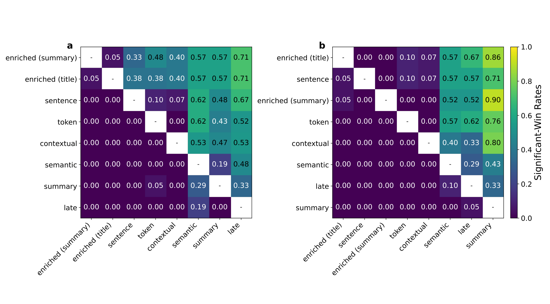
Figure 1 (Methods §3.2; original anchor S3.F1): The two panels show NDCG@10 and Recall@100. Each cell is the proportion of reported settings in which the row method significantly beats the column method. The 0.71 in the NDCG panel means Enriched (Summary) significantly beats Late in 71% of settings; it is neither a 71-percentage-point quality gain nor a 71% chance of improvement on a new query. This is the original figure by Caspari et al., reused under CC BY 4.0; the image is retained without cropping or redraw.

The matrix answers “across how many comparison settings was a significant win observed?” It is not an absolute probability of winning on all traffic. Enriched (Summary) fares better against several methods under NDCG@10, suggesting that document-level context can sometimes improve top-rank ordering. But it rarely beats Enriched (Title), and its advantage is weaker under Recall@100. Token and Sentence therefore remain competitive for first-stage candidate retrieval.

Read the rankings in terms of the service stage. If a reranker consumes the first hundred candidates, a small lead in top-ten ordering may matter less than candidate coverage. If the search interface presents the top ten directly, NDCG@10 may be more relevant. This is an engineering interpretation of the metric definitions, not a claim that the paper mandates one metric for a particular architecture.

Evidence 2: Table 2 gives conditional results, not one grand ranking

Table 2 in Results §4 reports Recall@100 for selected model, corpus, and scale combinations. The following CoRE slices help show how rankings move. Higher scores are better; these values illustrate dependence on setting and do not, by themselves, establish statistical significance.

Model and scale	Token	Sentence	Enriched (Title)	Enriched (Summary)
Gemma × CoRE, 10K	82.73	82.55	82.55	82.36
Gemma × CoRE, 1M	57.09	56.00	57.27	55.64
Qwen × CoRE, 10K	76.73	76.18	78.00	77.45
Snowflake × CoRE, 10K	77.64	79.09	78.18	78.91

As Gemma × CoRE grows from 10K to 1M, the relative positions of Token and Enriched (Title) change; for Snowflake at 10K, Sentence leads. These are only a few rows from Table 2, but they show why no method stays on top across every embedding model and corpus scale. Table 2 marks the highest and second-highest scores; rank alone is not a pairwise significance test. Read the table with Figure 1, which aggregates significant comparisons across settings.

The authors also observe that the number of significant differences generally increases as the corpus grows, but not monotonically: the largest KILT setting, at about 6M documents, has fewer significant differences than the 1M setting. A larger corpus does not make every strategy gap grow proportionally. Models, data slices, and query samples still shape the results. The authors publish fuller tables in the evaluation repository’s results.md.

Evidence 3: Figure 2 exposes indexing, query, and memory costs

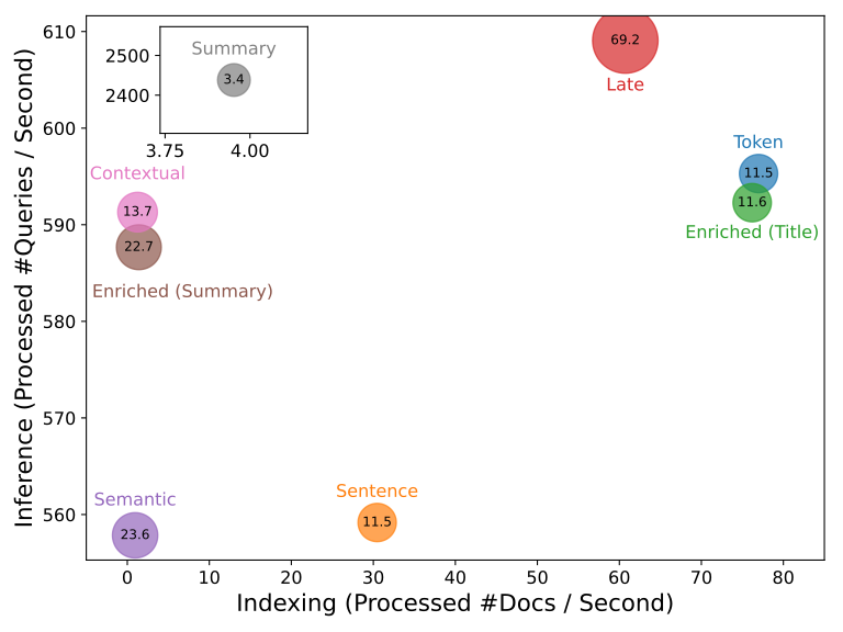
Figure 2 (Results §4; original anchor S4.F2): This plot covers only Gemma × KILT 10K. The x-axis is documents processed per second during indexing; the y-axis is queries per second; circle size represents RAM during index construction. Summary-only appears in an inset because its query throughput is higher and would compress the differences among other points. This is the original SVG by Caspari et al., reused under CC BY 4.0 without crop or redraw.

In this setting, Token has higher indexing throughput and relatively low memory. Sentence is slower to build despite its conceptual simplicity. Semantic, Contextual, and summary-based methods index more slowly because they require additional sentence encoding or summary/context generation. Summary-only uses one summary representation per document, which gives it higher query throughput but lower retrieval effectiveness and costly document processing. Late retains unpooled token representations before final chunk embeddings, increasing peak indexing memory in this experiment.

Figure 2 is one runtime slice, not a universal cost curve for eight methods or all hardware. Changing the embedder, batch size, FAISS index, hardware, or generation service can alter absolute values and relative costs. The figure is most useful as a reminder to record all three cost dimensions, not as a throughput number to copy into a cloud-cost estimate.

Table 3 in Results §4 expresses document throughput for Contextual and Summary as a function of generation throughput. At average LLM output rates of 100, 200, 500, and 2,000 tokens/s, Contextual corresponds to about 0.26, 0.53, 1.31, and 5.26 documents/s; Summary corresponds to 0.77, 1.57, 3.93, and 15.74 documents/s. These are document-rate estimates conditional on output speed, not measured benchmarks across multiple generation providers. The paper also estimates a provider-dependent US$9.60–14.73 cost for Contextual on KILT 10K using OpenRouter prices at the time of writing. That is a time-specific example, not a current quote or a cost projection for a larger corpus.

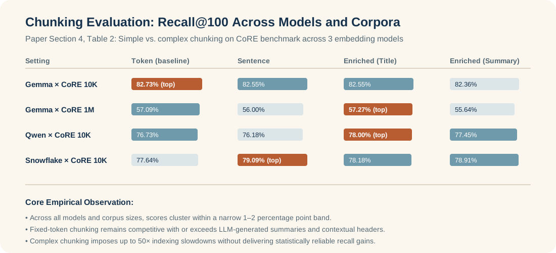
Figure 3 (Results §4; summary derived from Table 2, original anchor S4.T2): Visualizes Recall@100 across models and scales. Strategy scores cluster within 1–2 percentage points, with simple Token matching or outperforming complex generative summaries in several settings, demonstrating that expensive chunking lacks a consistent recall advantage. Reused and formatted under CC BY 4.0.

Bloss0m engineering judgment and when not to use it

Paper result: In the tested settings, expensive methods rarely deliver consistent gains over simple chunking. Different methods can achieve similar retrieval scores while using different indexing throughput, query throughput, and memory. The authors describe Token as a strong baseline for many large-scale retrieval settings, Sentence as an alternative when sentence boundaries matter, and Enriched (Title) as a low-cost candidate when useful titles exist. Enriched (Summary) performs well in some NDCG@10 comparisons, but the authors recommend comparing it with the cheaper Title version. Semantic, Contextual, Late, and Summary-only are better treated as candidates for specific requirements than as default upgrades.

Bloss0m engineering synthesis: Compare chunkers as design points rather than rank them on a single “complexity” ladder. A small local benchmark can follow this sequence:

1. Choose the service stage and objective. Say whether the index supports direct top-ten ranking, candidate recall before a reranker, or another task. Select the primary metric accordingly and keep any secondary metric needed to reveal trade-offs.
2. Hold data and queries fixed, then compare inexpensive baselines. Start with Token, Sentence, and Enriched (Title), then add one expensive method with a specific hypothesis. If testing multiple embedding models, report them separately so averages do not hide interactions.
3. Record quality and cost together. Track NDCG or Recall, indexing throughput, query latency or throughput, peak memory, vector count, generated tokens, and rebuild cadence. Figure 2 covers one small setting; the target workload needs its own measurements.
4. Require incremental value to pay for incremental cost. Promote an expensive method to a default only when its gain remains stable across reruns and fits update, latency, and resource budgets. If several objectives are collapsed into one score, derive the weights from product needs rather than letting the paper choose them implicitly.

This sequence is a Bloss0m engineering synthesis, not a formal algorithm or utility function proposed by the authors. For a service with a hard latency SLA, throughput may be a constraint rather than a score that can be traded against quality. For a frequently updated corpus, rebuild time may matter more than one-time index speed. Those conditions have to be measured in the actual pipeline.

Limitations and evidence boundary

First, runtime and memory depend on the authors’ implementation, hardware, batching, and FAISS configuration. They support comparisons within that setup, not universal cross-platform cost constants. Second, CoRE and KILT/NQ cover particular corpora, query styles, and relevance judgments; they do not represent every internal enterprise corpus, multilingual collection, codebase, table-heavy PDF, or permission-filtered search system. Third, Contextual is evaluated only up to 100K documents on CoRE and 1M on KILT. Its quality and cost at larger full-corpus scale cannot be inferred from those results. Fourth, the authors hold some chunking parameters fixed for comparability rather than exhaustively tuning each strategy, so the study is not a contest of every method’s best attainable configuration.

The experiments measure retrieval, not the generator’s final answer correctness, citation quality, or user-task success. A reported improvement in NDCG@10 cannot be rewritten as improved end-to-end RAG quality. Summary-only’s higher query speed alone also does not show that it suits a specific product. If internal titles are poor, documents change frequently, or the language and relevance-label distribution differ, the benchmark must be rechecked on target data; aggregate results provide no guarantee of external validity.

Artifacts and reproducibility

As of September 26, 2026, the authors’ chunking-eval repository is publicly browsable and its README provides setup and evaluation instructions; GitHub repository metadata does not declare a code license. The linked KILT-NQ and CoRE Hugging Face datasets are currently public and ungated, with corpus, query, and relevance-judgment files listed. Their API metadata does not state a dataset license. The repository notes that EmbeddingGemma requires accepting its model license. Public endpoints do not mean that every large file has been downloaded, nor that the code and data share one license.

The measurements in this article are the authors’ reported results, not an independent reproduction. The README documents uv setup and command-line evaluation examples; before attempting a larger run, check the chosen corpus split, model terms, disk capacity, and compute resources. To compare Table 2 or Figure 2, also record repository, dataset, and model revisions, chunk settings, FAISS parameters, and hardware. Without those conditions, a rerun need not reproduce every number exactly.

Three things to remember

1. Technical idea: Chunking changes searchable units, vector count, and system cost; it is more than a text-preprocessing choice.
2. Strongest evidence: Figure 1 shows that NDCG@10 and Recall@100 produce different method rankings; Table 2 and Figure 2 show how data settings and cost dimensions affect the choice.
3. Adoption boundary: Simple methods are reasonable starting points. Expensive methods should earn their place on the target data, metric, and indexing budget.

Further reading and primary sources

• RAG-ANYTHING: Can one retrieval method serve a multimodal knowledge base?: retrieval trade-offs when searchable units extend beyond plain text.
• RAG-MCP: Reducing context for tool selection: compare indexing and recall when the retrieved objects are tool descriptions.
• Paper v1 HTML · v1 PDF · arXiv abstract and version history
• Authors’ evaluation code · KILT-NQ dataset · CoRE dataset