Does a Correct RAG Answer Mean the System Behaved Correctly? Reading The RAT

The paper in 90 seconds

• Problem: A final-answer score cannot tell whether a RAG system guessed correctly without evidence, refused despite having evidence, or changed its answer quality with retrieval state. The RAT asks whether a probability model can preserve these dependencies instead of compressing them into one mean score.
• Core insight: The authors represent retrieval $R$, abstention $A$, and task success $T$ as binary variables, factor their joint distribution according to the pipeline, $P(R,A,T)=P(R)P(A\mid R)P(T\mid A,R)$, and derive generator success $G$ as a deterministic function of those variables under a stated policy. Bayesian inference carries uncertainty through the derived quantity.
• Strongest evidence: Across 27 dataset–retriever–generator configurations, the three generators on Natural Questions (NQ) with dense retrieval have task-success estimates of only 0.239, 0.242, and 0.243, while their estimates of $P(G=1)$ are 0.164, 0.414, and 0.496. Under this operational policy and dataset setup, similar marginal task scores do not imply similar responses to retrieval failure.
• Main boundary: $G$ depends on the authors’ policy—abstain when retrieval fails and answer correctly when it succeeds. It is not a universal safety or quality truth. The study covers three KILT tasks, three retrievers, three 8–12B open-weight generators, a constrained retrieve-then-generate setup, and a binary all-or-nothing retrieval state.

Bounded verdict: The RAT does not claim to identify the causal root cause of a wrong answer. Its value is to quantify “correct answer” separately from “appropriate behavior given available evidence,” and to direct scarce labels toward a chosen estimand. If the policy, annotations, or judge calibration do not fit the application, a precise posterior can still answer the wrong question precisely.

Version, question, and claim boundaries

This reading follows arXiv v1 of The RAT: A Unified Bayesian Model for RAG Evaluation. The arXiv record lists Pius von Däniken, Felix Matthias Saaro, Mark Cieliebak, and Jan Milan Deriu; it was submitted to cs.CL on 2026-08-25. As of 2026-09-24, it is a preprint, not a peer-reviewed result. The reading covers the full v1 HTML, the version-pinned v1 PDF, Sections 1–6, Appendices A–G, Tables 1–11, and Figures 1–3 used below. The arXiv v1 page lists CC BY 4.0; the three original figures retain their content and are captioned with version, section anchor, and license. Independent inspection of the author-linked vodezhaw/rat repository indicates: As of 2026-09-24, GitHub lists a single README containing “Under construction…” and no code, data, release, or runnable instructions. “The paper is accessible” and “the method is reproducible” are different states.

This is a Bayesian evaluation-method paper with an empirical comparison. The reader’s question is not “Which retriever or model is the best in the world?” It is: when systems reach similar answer correctness, do they use evidence, choose to abstain, and avoid unsupported answers in similar ways? The authors argue that component-level benchmarks, end-to-end accuracy, and multi-dimensional evaluations reported independently may fail to preserve statistical dependencies among retrieval, abstention, and correctness. The RAT contributes a joint distribution factorized under its pipeline assumptions, from which it estimates marginal quantities, conditional behaviors, and a policy-adherence quantity.

Claim layer	Boundary used in this reading
Proposed by the paper	Section 3’s binary variables, joint-distribution factorization, deterministic definition of $G$, five base probabilities, and noisy-judge extension.
Evidence reported by the authors	The 27 configurations in Sections 4–5, conditional probability tables, 500 annotation subsamples, information-gain analysis, HotpotQA judge calibration, and Appendix C’s ternary partial-retrieval analysis.
Not established by the evidence	A universal policy for every RAG application, production improvements, causal root-cause identification, cross-domain validity, full reproducibility, or replacement of human labels by a judge.
Bloss0m engineering judgment	Treat $R/A/T/G$ as an example evaluation schema. Reuse requires redefining retrieval success, response policy, labels, and judge calibration while retaining production-specific failure dimensions.

Paper Essence Contract

1. Problem: A final RAG score compresses whether evidence was present, whether the generator followed an evidence-conditioned policy, and whether the answer was correct, making diagnosis ambiguous.
2. Why prior approaches are insufficient: Measuring retrieval or answer correctness alone does not describe how a generator’s behavior changes with retrieval state; equal task scores can come from different abstention policies.
3. Core idea: Model the dependence among $R,A,T$ jointly with Bayesian inference, then derive $G$ from an explicit policy. Marginalize unobserved labels rather than discarding every partially labeled example.
4. End-to-end mechanism: For a fixed query × retriever × generator, record retrieval success, abstention, and answer correctness; fit the posterior under the conditional factorization; derive $G$ from posterior draws; compare conditional probabilities, intervals, or annotation strategies.
5. Supporting evidence: The 27-configuration experiment contains near-equal marginal task scores but different $G$ values. HotpotQA + hybrid subsampling and information-gain analyses show that $R$ carries more information for the specified $G$, while $T$ carries more information for task success. Tables 4–5 expose false-positive problems for the judge setup studied.
6. Adoption boundary: $G$ is not a decision truth if the policy is inappropriate. Binary all-or-nothing retrieval, a controlled Wikipedia-derived corpus, single-turn tasks, exact-string abstention, a small model set, and an unreproducible artifact limit transfer.

Core intuition: correct answers and appropriate behavior are separate questions

Imagine two RAG systems that each answer 60 of 100 questions correctly. System A might say “I don’t know” when its documents lack an answer and respond accurately when support is available. System B rarely abstains, sometimes guesses correctly without evidence, and misses other questions for which evidence was present. An end-task score gives them the same result, although their evidence-sensitive behavior differs. This is a hypothetical teaching example, not an experimental case in the paper.

The RAT first defines the random variables: $R$ for retrieval state, $A$ for whether the model abstains, and $T$ for task correctness. It then derives $G$ from a policy. Bayesian inference is used to carry posterior uncertainty through the model and to integrate over unobserved labels instead of dropping all partially labeled records. This is a modeling choice. Although the factor order follows the RAG information flow, it does not prove causal effects of $R$ on $A$ or $T$. A conditional association such as $P(A\mid R)$ is not an intervention; datasets, prompts, models, queries, and evaluators may also shape the observed distribution.

Concept map: retrieval, abstention, answer, and policy success

Symbol	Operational definition in the paper	What it must not be conflated with
$R$	1 means the retrieved context contains all information-bearing documents needed to answer; binary in the main analysis.	Not “at least one relevant passage was found,” nor a directly observable semantic-sufficiency truth.
$A$	1 means the generator abstains using the prescribed explicit string; detected by exact matching in the experiments.	Not every natural-language hedge, cautious answer, or expression of uncertainty.
$T$	Whether the answer matches the task reference. The experiment treats abstention as $T=0$.	Not evidence support; the model can guess correctly when $R=0$.
$G$	Under the authors’ deterministic policy, abstain when $R=0); answer correctly when$R=1).	Not causal attribution, calibration, general helpfulness, or universal safety.

These distinctions matter. $T=1$ does not show that the response was supported by retrieved context; it may be a lucky guess. Conversely, if retrieval succeeded and the generator still abstained, $T=0$ and this fixed policy also yields $G=0$. The measure evaluates generator behavior relative to a specified policy; it is not simply answer accuracy with a new name. Nor does the model decide whether that policy is appropriate. If the policy is wrong, an accurate estimate can still give a misleading score.

Method mechanism: from a joint distribution to derived G

The authors factor the joint distribution according to pipeline information flow:

$P(R,A,T)=P(R)P(A\mid R)P(T\mid A,R).$

Read this as: first there is a retrieval outcome; conditional on that state, there is an abstention probability; finally, task success is described given both retrieval and abstention. This is a factorization of a joint distribution. It does not require a RAG runtime to execute three Bayesian modules in sequence, and it is not a structural causal model. Its advantage is that each parameter maps to an interpretable behavior:

• $\theta_R=P(R=1)$: retrieval-success probability for this configuration.
• $\theta_{A^-}=P(A=1\mid R=0)$: probability of abstaining after retrieval failure.
• $\theta_{A^+}=P(A=1\mid R=1)$: probability of abstaining despite successful retrieval.
• $\theta_{T^-}=P(T=1\mid A=0,R=0)$: probability of a correct answer when responding without complete retrieval.
• $\theta_{T^+}=P(T=1\mid A=0,R=1)$: probability of a correct answer when responding with complete retrieval.

Under the authors’ policy, generator success is:

$G=\bigl((R=0)\land(A=1)\bigr)\lor\bigl((R=1)\land(A=0)\land(T=1)\bigr).$

For the four $(R,A)$ combinations, $R=0,A=1$ is “no evidence, abstain”; $R=0,A=0$ is “answer despite missing evidence”; and $R=1,A=1$ is “evidence available, but abstain.” Only $R=1,A=0$ also requires checking whether $T$ is correct. This definition turns a selected policy into a derived probability, but it remains a measure of adherence to that policy—not a normative rule inferred from the data.

The authors use independent uniform priors for the five base probabilities and a Dirichlet prior for conditional judge outcomes. They use Stan with Hamiltonian Monte Carlo / NUTS; each experiment uses five chains, 2,000 warmup iterations, and 10,000 posterior samples per chain. A derived quantity such as $P(G=1)$ can be computed for each posterior draw, so its interval reflects finite labels and uncertainty within the model assumptions. More samples do not automatically correct a misspecified construct, prior, likelihood, or label.

Worked example: one query through the model (illustrative)

The following is a Bloss0m-created explanation, not a paper observation. Suppose a user asks, “Has this procurement completed its security review this year?” The retriever returns documents but none includes the review result; the product policy says to abstain unless complete evidence is available. One record moves through the paper’s variables as follows:

1. Input: A fixed query, retriever, generator, and corpus snapshot—in this example, the procurement question above.
2. Intermediate state $R$: The evaluator checks whether every document defined as necessary is present in the retrieved context. If a required result is missing, the main analysis records $R=0$; retrieving some relevant text does not change this all-or-nothing label.
3. Model decision $A$: If the output exactly matches the prescribed abstention string, record $A=1$. Otherwise, record $A=0$. Under this protocol, “I’m not sure, but it may be complete” may not count as abstention.
4. Outcome $T$: For a non-abstaining response, compare it with the reference answer. A string-correct answer can yield $T=1), even though it does not prove that retrieved evidence supported it.
5. Derived $G$: If $R=0,A=1$, the response follows this policy. If $R=0,A=0), then$G=0$even if the guess happens to be correct. If$R=1,A=0), $G=1$ only when $T=1$.
6. Likely failure point: Does the gold retrieval label represent sufficiency? Does the product policy permit a partial answer? Did exact-string matching miss a natural abstention? Any one of these can change how the posterior should be interpreted.

This walkthrough explains how one record enters the model. It does not interpret the observed conditional distribution as “retrieval failure caused abstention,” and it does not make $G$ a substitute for product policy, safety review, or human judgment.

Paper Figure 1: dependency structure, not causal proof

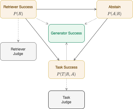
Figure 1, from arXiv v1 Figure 1, appears in Section 1. Notice how $R$ conditions the model and how $G$ is derived from retrieval state, abstention, and task outcome. This is a dependency diagram for the paper’s evaluation construct, not a causal DAG or a runtime architecture that systems must execute. Reused under CC BY 4.0 as listed on the arXiv v1 page; the local image is neither redrawn nor cropped.

Building the experiment: a controlled comparison of 27 configurations

The authors use FEVER, HotpotQA (HQA), and Natural Questions (NQ) from KILT, sampling 10,000 queries from each task. They combine documents relevant to those queries into a shared Wikipedia-derived knowledge base of 1,720,160 paragraphs. Most FEVER queries have one relevant paragraph and use the labels SUPPORTS, REFUTES, or NOT ENOUGH INFO; HQA has two relevant paragraphs per query and requires multi-hop reasoning; NQ uses short-answer annotations and is also defined with one relevant paragraph per query. This supports comparison across different evidence burdens, but it remains a controlled corpus rather than a production collection.

Three retrievers are tested: sparse retrieval using BM25, dense embedding retrieval indexed with HNSW/FAISS, and hybrid retrieval using Reciprocal Rank Fusion. Each returns the top five passages. The generators are Apertus 8B, Gemma3 12B, and Qwen3.5 9B, yielding 3 datasets × 3 retrievers × 3 generators = 27 configurations. Outputs are constrained by prompts to a short answer or exact abstention string. That makes labels easier to observe but narrows the answer format on which the results depend.

Paper Figure 2: which variable should a limited budget label?

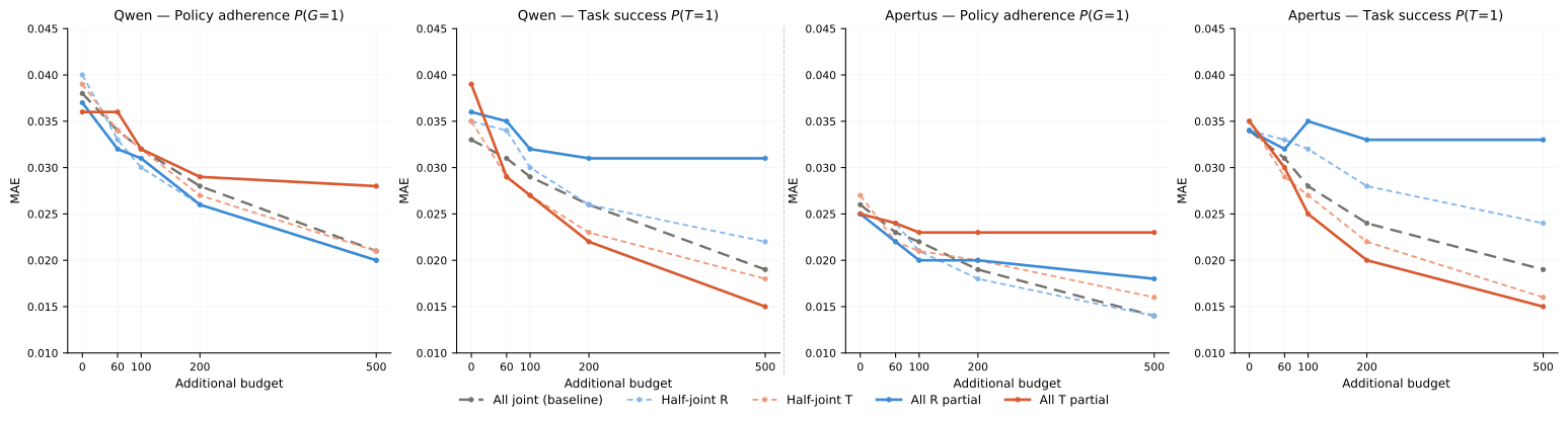
Figure 2, from arXiv v1 Figure 2, is in Section 5.3. It compares five added-label strategies for Qwen and Apertus on HotpotQA + hybrid retrieval, starting with 100 fully labeled baseline records, observable string-matched abstention, and different added budgets, averaged over 500 subsamples. The lesson is that the best annotation direction differs for $G$ and $T$, not that “retrieval labels are always better.” Reused under CC BY 4.0 as shown on the v1 page; the original SVG is used without changing data or axes.

Each annotation experiment starts with 100 base samples labeled for both retrieval and task success; abstention is assumed observable from the output string. An additional budget of 60, 100, 200, or 500 samples is split among all-joint, half-joint-R, half-joint-T, all-R, or all-T strategies. The authors resample 500 times from 10,000 task examples and calculate MAE and 95% credible interval width against a full-data point estimate. This sub-experiment uses HQA, the hybrid retriever, Apertus, and Qwen—not all 27 model configurations.

For this fixed target, retrieval-focused labels typically reduce error faster for estimating policy adherence $P(G=1)$; for $P(T=1)$ the direction reverses, because task labels directly observe the target. All-joint is a robust option for both when the eventual estimand is not known in advance, since it does not rely on information omitted by one target-specific strategy. This is a clue for annotation design, not a claim that retrieval labels are universally cheaper or more valuable than task labels.

Why does a retrieval label carry more information about G?

Table 3 and Appendix F explain the structure. When $A$ is observed, three of the four $(R,A)$ cells determine $G$: retrieval failure plus abstention is success; retrieval failure plus an answer is failure; and successful retrieval plus abstention is also failure. Only successful retrieval plus an answer still requires $T$. Therefore, observing $R$ resolves $G$ directly for more cases than observing $T$ alone.

For HQA + hybrid, the information gain per sample is 0.526 for all-joint, 0.436 for half-joint-R, 0.345 for all-R, 0.340 for half-joint-T, and 0.154 for all-T with Qwen. With Apertus, the corresponding values are 0.490, 0.387, 0.284, 0.345, and 0.200. These are information-gain calculations using estimated probabilities for that configuration, not annotation ROI rankings that can be copied across models and policies. The authors also observe that Qwen’s all-R strategy can empirically edge out all-joint at larger budgets, despite lower per-sample information gain. The initial 100 joint labels already constrain the one ambiguous cell requiring $T$, so later joint labels have diminishing returns. This is a useful warning: an information-theoretic ranking does not replace finite-sample behavior.

Paper Figure 3: inspect posterior intervals as well as error

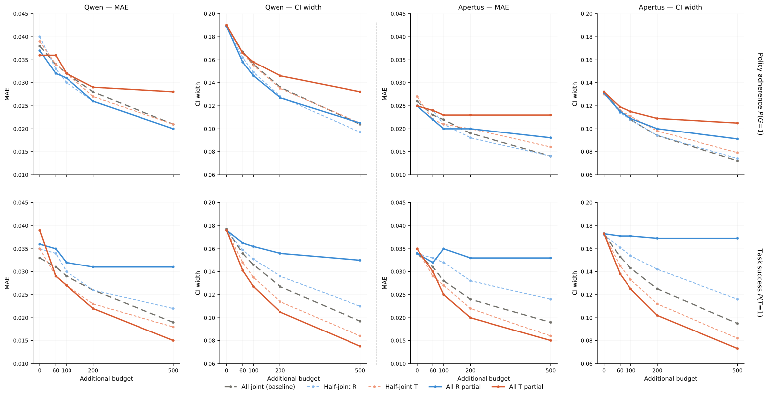
Figure 3, from arXiv v1 Figure 3, is in Appendix E. The top row is $P(G=1)$ and the bottom is $P(T=1)$, with both MAE and 95% credible interval width. At budget 500 for Qwen, the $P(G=1)$ interval width is 0.105 for all-R versus 0.132 for all-T; for $P(T=1)$ it is 0.075 for all-T versus 0.150 for all-R. The appendix figure extends the main-text MAE-only Figure 2 and makes the target-dependent reversal visible. Reused under CC BY 4.0 as listed on arXiv v1; the original SVG is unchanged.

For the same 500-budget example, the authors report coverage close to nominal 95% across strategies; all-joint maintains narrow intervals for both targets. Do not confuse a credible interval with query-to-query variability or uncertainty across production deployments: it is a posterior interval under this Bayesian model, data, and sampling setup. Useful uncertainty quantification still depends on whether the variables, priors, and observation model fit the application.

The clearest comparison: near-equal task scores, different policy behavior

Table 1 gives marginal outcomes; Table 2 decomposes conditional probabilities. The clearest contrast is NQ + dense: Apertus, Gemma3, and Qwen3.5 have $P(T=1)$ values of 0.239, 0.242, and 0.243, nearly overlapping, while $P(G=1)$ is 0.164, 0.414, and 0.496. Table 2 also shows different abstention estimates under retrieval failure: $P(A=1\mid R=0)$ is 0.039, 0.382, and 0.513. The accurate interpretation is that the three models have different estimated behaviors under the policy and combination of data, retriever, and prompt studied. It does not show that Qwen3.5 is “safer” across real-world RAG systems.

The HQA + hybrid conditional estimates make the same point more concrete. Apertus abstains with probability 0.039 after retrieval failure and 0.005 after success; Gemma3’s figures are 0.270 and 0.021; Qwen3.5’s are 0.463 and 0.036. Read this as “the observed abstention probabilities differ with retrieval state and model,” not “retrieval caused the model to refuse.” The paper does not randomize a retriever intervention to identify a causal effect. Instead, it uses conditional distributions to describe behavior within its experimental setup.

There is also a dataset-dependent trade-off: hybrid has the highest marginal retrieval success on FEVER and NQ, whereas sparse is best on HQA. FEVER’s answer space has only three labels and most queries need one document, so task success is naturally higher. Teams should not equate a retrieval leaderboard with a downstream answer win, or compare raw success across datasets as if they had the same difficulty. The RAT makes dimensions visible but does not choose the team’s utility function.

LLM-as-a-judge: modeling noisy labels does not make them gold

The authors use GPT-4o-mini to estimate retrieval and task labels, introducing $R_J$ and $T_J$ as noisy observations of the ground-truth variables and building a calibration likelihood from Table 4’s TPR/FPR. The extension lets human and judge labels coexist while propagating calibration error; it does not claim the judge self-calibrates into ground truth. Judgments still depend on prompts, benchmark, and calibration sample.

On HQA, the retrieval judge has TPR 0.77 and FPR from 0.17 to 0.19 depending on retriever. The task judge has TPR from 0.88 to 0.94, but FPR from 0.32 to 0.43. Since actual task success is around 0.21, the false positives substantially inflate observed judge success: Table 4’s $P(T)=0.21$ corresponds to $P(T_J)$ around 0.52–0.57. This is a base-rate-sensitive operational lesson: reporting judge accuracy or TPR alone can hide false positives when the positive class is uncommon.

Table 5 starts with 200 fully human-annotated samples and adds 0, 500, or 5,000 automated judge annotations. For HQA + hybrid + Apertus, the 95% interval width for $P(G=1)$ declines from 0.0941 to 0.0802, while MAE stays around 0.017. For $P(T=1)$, interval width moves from 0.1246 to 0.1150 and MAE remains around 0.023. Five thousand noisy annotations narrow some intervals, but do not yield a corresponding clear MAE improvement. This is an author experiment with one judge and a specific calibration setup, not evidence that every judge is useless. The engineering question it supports is: measure calibration and false-positive behavior before scaling automated labels.

Appendix C matters: partial retrieval is folded into failure by the main model

The main model defines retrieval success as having all needed documents in context. A query with some necessary evidence retrieved is therefore binarized as $R=0$. Appendix C adds a separate three-state analysis: fail / partial / success. HQA has two relevant paragraphs per query, and its partial-retrieval rates are 47.24% for dense, 56.47% for hybrid, and 52.33% for sparse. FEVER ranges from 3.00% to 4.53%; NQ is 0% because each query has one relevant paragraph.

This appendix sees abstention decrease and task success increase as retrieval quality increases in HQA, consistent with the main-text direction. But the paper does not turn the ternary version into a full new policy model, nor solve the issue that relevance labels may not capture which passages are individually sufficient versus jointly necessary. Partial retrieval is thus a warning and a useful slice for the main model’s external validity; it is not a completed solution to fine-grained retrieval quality.

Experimental context and evidence map

Question	Controls and measurement	Location and limitation
What are the marginal outcomes across 27 configurations?	3 KILT datasets × 3 retrievers × 3 generators; top-5 retrieval; report $P(R)$, $P(A)$, $P(T)$, and $P(G)$.	Table 1; the query-derived shared Wikipedia corpus and constrained answer format do not form an open-web production benchmark.
Do similar task scores hide different conditional behavior?	Fit the Bayesian model per configuration and estimate $P(A\mid R)$ and $P(T\mid A,R)$.	Table 2 supports within-setup conditional differences, not causal attribution or cross-domain transfer.
How should a scarce annotation budget be allocated?	100 joint base labels + 60/100/200/500 additions; five strategies; 500 subsamples; Qwen/Apertus on HQA + hybrid.	Figures 2–3, Table 3, Appendices E–F show target-dependent error and uncertainty.
Do noisy judge labels help?	GPT-4o-mini judges; calibrate TPR/FPR on human labels; add 0/500/5000 judgments; main report for HQA + hybrid + Apertus.	Tables 4–5 show high FPR and limited gains under this setup; judge/model coverage is narrow.
What does binary $R$ hide?	Appendix C separates fail / partial / success.	Tables 8–9 show partial retrieval concentrated in HQA; relevance annotation and policy simplification remain.

Directly supported by the paper: the variable definitions, 27 configurations, inference model, conditional tables, annotation subsampling, judge calibration, partial-retrieval tables, and their stated settings and values. Author interpretation: conditional decomposition makes differences visible when marginal task scores are near-equal; observing $R$ is more informative for estimating the specified $G$ in this design; judge FPR limits the marginal value of noisy labels. Not established: that RAT improves production answer quality, identifies causal root causes, provides a universal policy, makes a judge a human replacement, or is currently reproducible from the linked artifact. Bloss0m judgment: reporting outcome and policy behavior separately can help internal evaluation, but $G$ must be reviewed alongside business risk, partial-answer allowances, cost, and escalation policy.

Failure modes and adoption limits

1. Binarization discards gradations. Retrieval may find some evidence, weak support, or conflicting passages; the main model uses fail/success. Continuous or ranked IR views such as MRR and MAP do not map automatically onto the current binary construct.
2. $G$ encodes a policy choice. The paper fixes “abstain on retrieval failure; answer correctly on success.” If an application permits a qualified partial answer, different abstention thresholds, or risk-specific policies, $G$ must be redesigned. Do not use the published definition to rank systems by default.
3. Retrieval success depends on the gold definition. The authors call retrieval successful only when all relevant documents are present. For questions answerable from one passage but labeled with several relevant passages, this can mark an answerable context as failed; conversely, sufficient evidence absent from the gold list may be missed.
4. Abstention uses exact matching. This works for a constrained single-answer prompt but misses free-form hedging, partial refusal, or indirect uncertainty. A production classifier would introduce another noisy measurement needing calibration.
5. Task, model, and pipeline coverage is narrow. Three benchmarks, three 8–12B generators, a retrieve-then-generate setup, and single-turn evaluation. Query reformulation, reranking, chunk filtering, iterative retrieval, and multi-turn memory add decision points not modeled here; extending the model requires new variables and validation of the factorization.
6. A shared corpus can make absolute retrieval look optimistic. The corpus is built from documents relevant to the selected queries and is more controlled than a fully open-domain collection. The authors note that absolute retrieval-success rates may therefore be optimistic; table values are not deployment-recall forecasts.
7. Posterior uncertainty does not include every model uncertainty. Credible intervals express uncertainty within the chosen model. If annotation validity, prior sensitivity, data drift, or omitted variables are not represented, the interval does not automatically absorb them.
8. The repository is not executable yet. Although the paper links a public GitHub repository, the inspected page contains only a placeholder README. Requirements, code/data completeness, license, release, and reproduction commands could not be verified; the artifact should not be called reproducible.

Bloss0m engineering judgment and when not to use it

The following is a Bloss0m engineering synthesis, not a product architecture or official checklist proposed by the paper. If a team wants a RAT-like decomposition, write an evaluation contract before looking at model scores:

1. Choose the decision policy. Under which evidence states may the system answer, answer partially, abstain, or escalate to a human? Define policy success before scoring; do not adopt the paper’s $G$ as an implicit default.
2. Make labels reproducible. Specify whether relevant evidence means “at least one sufficient passage” or “all labeled documents retrieved.” Handle partial and conflicting support, and test construct validity with blind double annotation or adjudication.
3. Separate estimands. Report task correctness, retrieval state, and abstention/policy behavior with denominators and conditional slices. A composite score alone is insufficient, but adding another metric does not by itself provide root-cause observability.
4. Name the target before spending on annotations. If the decision concerns policy adherence, measure the marginal information in retrieval labels; for answer quality, task labels observe the target directly. Use pilot subsampling to compare MAE, interval coverage, and human cost rather than copying Table 3’s ranking.
5. Calibrate automated judges. Keep a human gold slice; measure confusion matrices, TPR/FPR, and task slices separately for retrieval and task judgments. For low-prevalence outcomes, inspect false positives. If calibration drifts, do not treat a larger judge volume as an equal amount of valid evidence.
6. Keep other failure paths visible. RAT is a minimal schema. It does not include policy violations, faithfulness, citation validity, data permissions, latency, cost, multi-turn memory, or tool side effects; production monitoring needs additional dimensions matching actual risk.

The model is most plausible to try when references are stable, evidence sufficiency can be labeled consistently, and the policy is explicit. Do not apply it directly when free-form abstention is undefined, partial evidence is common but unscored, ground truth is missing, the judge is uncalibrated, or policy requires risk-sensitive trade-offs between abstention and partial answers. The RAT makes these questions visible but does not answer the normative decisions for a team.

Artifact and reproducibility (as of 2026-09-24)

• Primary paper: The arXiv v1 PDF, HTML, and source endpoints open directly; the version is dated 2026-08-25, and the page lists CC BY 4.0. This reading stays on v1 and does not combine claims from a later version.
• Code: The author-linked vodezhaw/rat is a public GitHub repository, but its file listing contains only a README with “Under construction…”. As of the check date, there is no runnable implementation, dataset, release, dependency lockfile, or reproduction instruction. Status: placeholder / not currently runnable, not “public code is available.”
• Data and outputs: The paper describes KILT subsets, a shared 1,720,160-paragraph corpus, and model conditions, but the inspected author repository contains no corresponding data, generated outputs, or environment manifest. Rebuilding the full process from official artifacts is unverified.
• Smallest reproduction path (conditional): If code, required KILT inputs, and model endpoints become available, fix one dataset × retriever × generator, create labels under Section 3, rerun the five-chain NUTS fit, and compare posterior summaries; then reproduce the HQA allocation experiment with 500 resamples. At present this is a plan inferred from the method description, not a successful reproduction.
• Open checks: When code will be filled in; corpus preprocessing and manifest; exact model checkpoints and decoding settings; priors and judge calibration data; chain diagnostics, compute costs, and seed sensitivity; transfer to partial/soft policies, multi-turn tasks, and open corpora.

Three things to remember

1. Technical idea: The RAT jointly models $R,A,T$ and derives $G$ from an explicit policy. Conditional structure complements one task score, but factorization is not causal proof.
2. Evidence: On NQ + dense retrieval, three generators have almost the same task success but different $P(G=1)$. HQA analyses show the relative value of retrieval labels for $G$ and task labels for $T$, while judge false positives make calibration essential.
3. Adoption boundary: Priors, annotations, and a binary policy determine the question the model answers. The linked GitHub repository remains a placeholder as of the check date, so the method can be read but not treated as a ready-to-run package.

For a next read, Causal Failure Attribution in Agentic RAG separates intervention-based causal attribution from ordinary failure diagnosis, reinforcing why this paper’s conditional dependencies should not be called root causes. Predicting Partial Answer Quality in Agentic RAG offers a different way to connect per-iteration answer quality with stopping decisions. Neither is a validated extension of RAT.

Primary sources

• von Däniken, P., Saaro, F. M., Cieliebak, M., & Deriu, J. (2026). The RAT: A Unified Bayesian Model for RAG Evaluation, arXiv v1. DOI: 10.48550/arXiv.2608.24753.
• Full HTML, version 1 (Figures 1–3, Tables 1–11, Appendices A–G).
• Author-linked RAT repository (placeholder README only as of 2026-09-24).