Refuse, Decompose, Refresh: Claim Boundaries in Closed-Loop AI Evaluation

The paper in 90 seconds

• Problem: In a closed-loop system, the evaluated policy helps determine which states are visited, which components receive traffic, and whether a failure leaves a recognizable trace. Even perfectly reproducible arithmetic may answer the wrong question if the policy never visits a state that would reveal a component’s behavior.
• Core insight: Treat evaluation as a claim contract. First establish whether the observations support the requested comparison. Then report execution integrity, operational false-admission safety, coverage, and structural hypotheses separately. When the distribution shifts relative to the detector’s reference, request a new reference map instead of calling the alarm evidence of a fault.
• Strongest evidence: In the authors’ aggregate-only simulator, affected clean traffic predicted stable detection better than the number of edited component cells. Across 540 unit-arm rows, the cell-minus-traffic negative-log-likelihood difference was 0.1264 nats per row, with a 95% interval of [0.0593, 0.1918] clustered over 20 physical components. This is a structural comparison among admitted units, not the diagnostic accuracy of a deployed agent.
• Main boundary: The experiment covers only 24 policy components, three demand regimes, two counterfactual fault masks, and aggregate traces. Its refresh check reuses the original reference buffer, so it cannot show that fresh data repair an obsolete map. It does not validate a live agent or localization accuracy.

This reading follows the arXiv v1 preprint submitted on September 17, 2026; peer-review status is not established. The paper starts from a question hidden by many benchmark scores: when the policy changes how the data are generated, what can a score actually represent? It also discloses a withdrawn comparison of exact minimum hitting set (MHS) and propagation-aware greedy selection. They agreed because scoped probes had already collapsed the residual choices, not because the analysis showed that either method was superior. This negative result motivated a formal held-out study of evidence eligibility and calibration instead of MHS superiority or localization accuracy (Section 1). The authors propose three actions—Refuse, Decompose, and Refresh—and instantiate them in a closed-loop simulator with explicit support gates, false-admission calibration, competing exposure measures, and reference-shift states. The held-out results support the protocol’s executability within that simulator. They do not show that the same thresholds work for real models, tool environments, or multi-agent systems.

What to know first: a score operationalizes a construct

An evaluation begins with a construct someone wants to understand—reliability, diagnosability, or safety, for example—and operationalizes it through tasks, observable variables, interventions, and metrics. The operationalization is not the construct itself. A metric can be computed exactly and a program can reproduce it bit for bit, yet the result may support a weak claim if the task did not expose the relevant behavior or the data did not support the comparison. A limitation of prior approaches is that broader scenario and metric portfolios still do not always ask whether each observation supports the requested comparison. In Section 2.1, the authors connect this issue to construct validity, benchmark overgeneralization, and overlap in high-dimensional comparisons. Their focus is an earlier gate: is there enough observable support to define the requested measurement in this case?

The estimand here is neither a treatment effect nor policy value. It asks whether a planted component intervention could produce a stable observable difference under traffic generated by the target policy (Sections 2.1 and 3.1). If the policy never visits the region affected by a fault, editing many cells may not change the aggregate trace. If demand shifts the traffic distribution, a comparison with an old reference may cease to be meaningful even when no fault was planted. These are different problems: one concerns whether the intervention can be seen; the other whether the reference still applies. They should not share one pass/fail field.

Core intuition: distinguish missing evidence from no detection

“Refuse” is not a low-confidence prediction abstention. It happens before the evaluator constructs a signal for a particular comparison. If a clean reference trace or a matched reference-current comparison lacks enough support, the comparison should not produce a diagnostic score. Only after a supported comparison fails to exceed the signal threshold can the result be NOT_DETECTED. At least three outcomes therefore remain distinct: not evaluated, evaluated with support but no detection, and evaluated with stable signal. Collapsing the first two into a zero score turns “unknown” into “measured zero.”

“Decompose” addresses a different mistake: combining unlike endpoints into one overall PASS. The protocol separates execution integrity, operational safety, descriptive coverage, structural hypotheses, and maintenance or refresh state. Each field answers a different question. A valid run does not make a research hypothesis true; high coverage cannot offset false admission; and a structural hypothesis passing does not mean every component was covered. The authors explicitly reject a single combined scientific label (Table 1, Section 4.4).

“Refresh” limits what a detector alarm means. If current traffic moves away from the frozen reference, an alarm can request invalidation and recomputation of the reference map. It cannot identify a failed component by itself. Fault-free current data may have shifted, and faulted data may remain close to the reference. In this paper, fault-null (no planted fault) and detector-null (matching the detector’s frozen reference distribution) are different concepts (Sections 2.3, 4.5, and 6.4).

Walk one example through the method: an intervention touches a high-traffic region

The example below follows the paper’s setup without adding new experimental numbers. Suppose the target policy sends some of a component’s traffic through cells that can be changed. The study uses two ways to select cells: uniform sampling among changeable cells, and flow-weighted sampling that favors cells with greater clean occupancy. The evaluator does not jump from the number of edited cells to a detection result. It checks observability and stability in stages.

1. Input and reference map: The simulator runs a target policy under demand regimes $\lambda_0\in\{5,7,9\}$. Its 24 disjoint policy components are represented in each of the three regimes, giving 72 regime-component units. Each unit has 15 partitions of aggregate trace summaries.
2. Reference support gate: A clean partition supports a component only when its existing support count is at least 12. A regime-component unit enters the reference map only if at least 14 of its 15 clean reference partitions qualify; otherwise it returns REFERENCE_ABSTAIN. The denominator is not silently reduced when evidence is sparse.
3. Matched runtime gate: To compare reference and current traces, both streams must meet support 12 in the same partition, and at least 14/15 matched pairs must qualify. Both outward and inward intervention directions must pass separately before they can be combined. Fourteen supported reference partitions plus fourteen supported current partitions are insufficient if they are different partitions.
4. Signal and state: For each matched partition, $z=\max(\mathrm{region\_d1}/0.20, |\mathrm{mean\_action\_gap}|/0.35)$. Development data selected the cutoff $z\geq1.50$ before the formal held-out run, and the threshold was not retuned on its null. A direction is stable when at least 14/15 partitions signal; unit-level stable detection requires both directions to be stable. Otherwise the unit can be eligible but not detected.
5. Output and likely misreading: The result separately records whether execution completed, whether the false-admission endpoint met its rule, where coverage existed, whether each structural hypothesis was estimable, and whether refresh was requested. Zero-occupancy faults form a separate stratum: they are not shifted by an arbitrary constant for log transformation and are not inserted into the primary modeling frame (Section 4.2).

If a unit fails either support gate, the method refuses before scoring. If support is adequate but stable signal is absent, the result is “not detected.” A likely failure point is that the support threshold is still an operational rule for this simulator: it may exclude rare but important components from the evaluated sample and may not fit a system without clean reference streams. Abstention makes unknowns visible; it does not remove selection bias automatically.

Experimental design: simulator, held-out data, and statistical units

The authors fit the target policy separately in three demand regimes. Each regime contains 24 disjoint policy components indexed by time quarter, inventory half, and market third. For each unit, the evaluator records 15 partitions of aggregate traces and does not inspect planted fault identity when determining eligibility or stable signal (Section 3.1). Formal interventions move changeable target-field cells by one action bucket. A uniform mask draws a seeded random ordering; a flow-weighted mask uses seeded weighted sampling without replacement based on clean occupancy (Section 3.2).

The study compares two operationalizations of fault size. cell_fraction is the selected-cell proportion, describing how much of a component’s definition was edited. Affected clean traffic is $\tau_d=\frac{\sum_{c\in S_d}o_c}{\sum_{c\in C}o_c}$, where $o_c$ is clean occupancy, $S_d$ is the selected fault subset for direction $d$, and $C$ is the component. The bidirectional traffic value averages the two directions. It asks how much clean policy traffic passes through the changed region; the cell fraction asks what share of the component’s geometry was changed. The same number of selected cells can affect different amounts of traffic. The comparison tests which measure better predicts aggregate signal opportunity; it does not prove a universal causal effect of traffic.

Development and formal held-out data use disjoint seeds. The held-out schedule covers five traffic targets, $\{0.15,0.30,0.50,0.75,0.95\}$, two mask families, three regimes, two directions, and 15 partitions. It contains 1,440 cases, 21,600 partition rows, and 3,456,000 simulated episodes. An episode is a Monte Carlo trajectory, not an independent statistical observation. Coverage starts with 72 regime-component units; safety and cluster-bootstrap inference use 20 represented physical-component clusters; and the main structural fit contains 540 rows—54 runtime-admitted units × 5 traffic targets × 2 mask families—nested within those clusters (Section 5). These denominators are not interchangeable.

The authors freeze three structural criteria. The traffic model must outperform the cell-fraction model in negative log likelihood, with the lower endpoint of the two-sided 95% cluster interval above zero. After adding mask family and its interaction with traffic, the one-sided 95% upper bound on log-loss gain must be below 0.01 nats per unit-arm row. Finally, total stable detections must not decrease across the five traffic targets in either family. Component-cluster bootstrap resampling uses physical components. These criteria were frozen for this study; they are not general evaluation standards.

Evidence map: what the three tables support

Figure 1 is a new Bloss0m layout based on the source’s Table 1. It is not an image of the paper’s table and adds no data; it makes the five independent output types and their inference boundaries easier to compare.

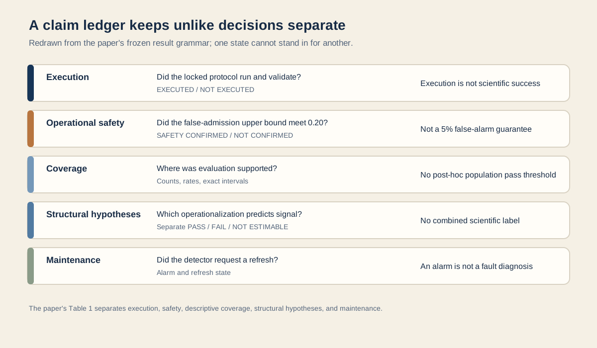
Figure: Bloss0m’s redraw of original paper Table 1 (Section 4.4). Execution, safety, coverage, structural hypotheses, and maintenance each have their own question and output; they should not be collapsed into one scientific PASS/FAIL. The content follows arXiv v1 Table 1. The source page lists the arXiv.org perpetual non-exclusive license. This is a new information graphic, not a copy of the paper’s table image.

The first finding is the coverage cost of refusal. In the held-out run, 55/72 regime-component units passed the reference gate, representing 20/24 physical components; 54/55 units then passed the two-stream runtime gate. Under independent reference evidence, reference-map invalidation was 0/20, with a two-sided exact 95% interval of [0.0%, 16.8%]. Runtime rejection occurred for 1/20 represented components, with an interval of [0.1%, 24.9%] (Section 6.1). The 17 clean-reference abstentions and one runtime abstention are outcomes. Forcing scores on them would rely on unverified extrapolation.

The second finding is a bound on operational safety. No represented physical component in the independent null arm crossed the stable-signal gate: zero events over 20 components. That zero does not mean zero risk. The one-sided exact 95% upper bound is 0.1391, below the study’s frozen operational tolerance of 0.20, so the authors label this endpoint SAFETY CONFIRMED. The 0.20 value is a threshold for this experiment, not a 5% false-alarm rate and not a guarantee for unseen component classes or shifted nulls. A finer, descriptive regime-component view reports 0/54, with an upper bound of 0.0540; it is not the primary sampling unit for the safety endpoint (Sections 4.3 and 6.2).

Figure 2 places two distinct endpoints side by side: support-gate coverage, and the denominator and upper bound for the safety endpoint. The values 55/72 and 54/55 describe the coverage path; 0/20 is a separate component-level safety sample and is not a downstream denominator on the same path.

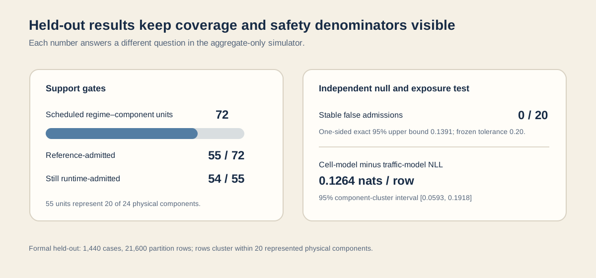
Figure: Bloss0m’s new held-out evidence graphic based on original paper Table 2 and Sections 6.1–6.3. The values 55/72 and 54/55 describe support coverage; 0/20 and its bound are a separate physical-component safety endpoint; 0.1264 comes from a model comparison over 540 nested rows. These are author-reported values, not new calculations. Source: arXiv v1 Table 2; the source page lists the arXiv.org perpetual non-exclusive license. This is an original Bloss0m visualization.

The main structural result favors affected traffic over cell fraction as a predictor of stable detection. The cell-model minus traffic-model NLL difference is 0.1264 nats per row, with a 95% interval of [0.0593, 0.1918] over 20 physical-component clusters; the interval is entirely above zero (Table 2, Section 6.3). At the same traffic target, flow-weighted masks often use fewer cells. After conditioning on traffic, adding family and the family-by-traffic interaction improves log loss by 0.0015 nats per row, with a one-sided 95% upper bound of 0.0066, below the frozen 0.01 criterion. This supports only a conditional claim: within the two mask families, traffic met this study’s practical-sufficiency endpoint.

That sufficiency result needs its fragility kept in view. The 0.01 margin is only 0.0034 nats above the observed upper bound, and the percentile cluster bootstrap has 20 represented components; finite-cluster undercoverage could favor the pass. A secondary traffic-plus-family coefficient has an interval of [-0.8617, 0.0367], corresponding to an odds-ratio interval of [0.42, 1.04]. Because its lower bound falls below the prespecified practical-equivalence range [0.5, 2.0], the paper does not establish coefficient-scale equivalence. The pass applies only to the log-loss sufficiency endpoint (Section 6.3).

Aggregate stable-detection counts also rise monotonically with traffic target: 0, 17, 37, 52, and 54 for uniform masks; 0, 13, 35, 49, and 54 for flow-weighted masks. This passes the frozen aggregate-monotonicity hypothesis, but only for admitted units, three regimes, two mask families, and this fault construction. It is not a causal law for every fault. This result and the traffic-versus-cell prediction comparison are related but distinct endpoints.

Failure pattern and reference drift: “clean” is not one null state

The authors use a separate drift log to examine reference-relative alarms. The detector’s frozen statistics came from development data in regime $\lambda_0=7$. All 45 current partitions were fault-null—no planted fault—with 15 in each regime. Pooled, the detector alarmed on 29/45 partitions, which can look like a 64% false-alarm rate if the reference definition is ignored. Stratification shows 15/15 alarms for demand-shifted $\lambda_0=5$, 0/15 for reference-matched $\lambda_0=7$, and 14/15 for demand-shifted $\lambda_0=9$ (Table 3, Section 6.4).

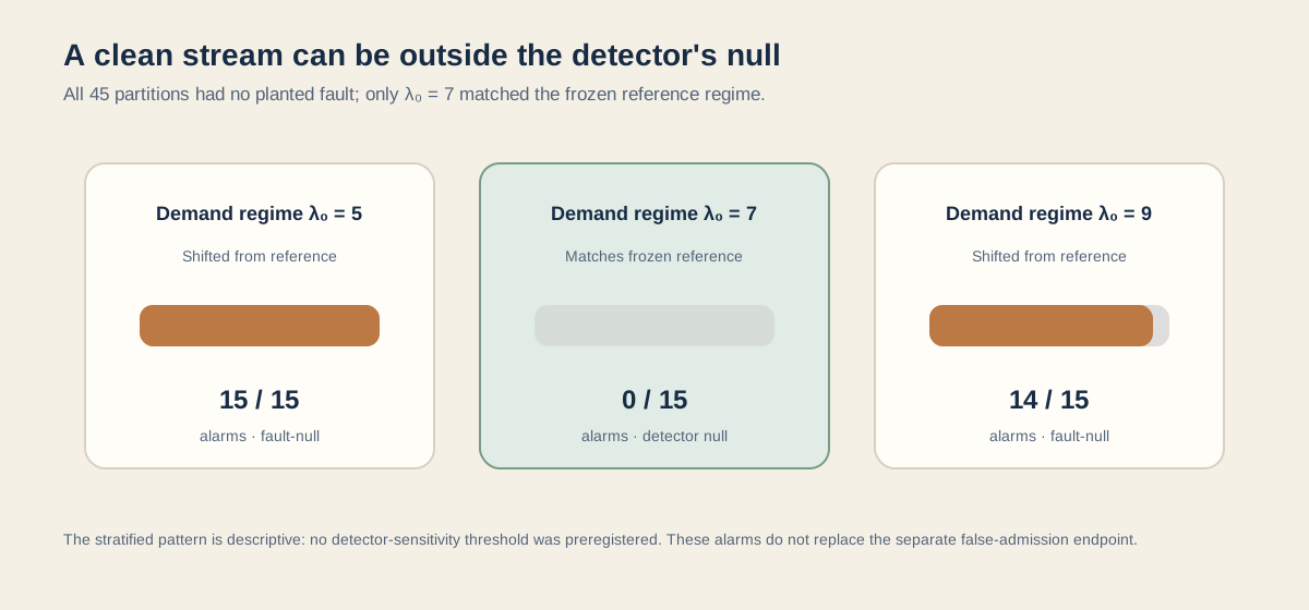
Figure: Bloss0m’s visualization of the alarm counts in original paper Table 3 (Section 6.4). All three rows are fault-null, but only $\lambda_0=7$ matches the detector’s frozen reference. Source: arXiv v1 Table 3; the source page lists the arXiv.org perpetual non-exclusive license. This is a new visualization of reported values, not a reproduction of an original figure.

The two outer regimes had no planted fault but did not belong to the detector’s reference null. Their alarms are consistent with the maintenance role “current conditions differ from the frozen reference; request a map refresh.” The paper did not preregister a detector-sensitivity threshold, so 15/15, 0/15, and 14/15 are descriptive regime slices, not a confirmatory sensitivity result. The preregistered stable false-admission endpoint in Section 6.2 is the relevant operational false-positive measurement. Drift alarms and stable fault admissions answer different questions, so 29/45 should not replace the 0/20 safety result.

The refresh endpoint is also narrow. After a detector requests an update, the protocol recomputes against the original locked reference buffer and checks whether the map hash returns to the expected value. Because the reference data are not replaced, this tests control flow and the hash invariant only. It cannot show that fresh data after genuine drift repair an obsolete reference map (Sections 4.5 and 9).

Evidence map: claims, held-out evidence, and what remains unknown

Question	Paper evidence	What the held-out result supports	What it does not support
Is the comparison supported?	Sections 4.1 and 6.1	Under the frozen gates, 55/72 reference units and 54/55 runtime units qualify; refusal belongs in the coverage report.	That all regimes and components are supported, or that these thresholds fit another system.
Is false admission below this study’s tolerance?	Sections 4.3 and 6.2	Zero stable false admissions among 20 represented components gives a one-sided 95% upper bound of 0.1391, below 0.20.	Zero risk, validity for unseen clusters, or a 5% false-alarm guarantee.
Which exposure measure tracks stable detection?	Section 5 and 6.3; Table 2	Among admitted data, the traffic model predicts better than cell fraction; adding family meets the 0.01 log-loss rule within two specified mask families.	That cell counts never matter, or coefficient-scale equivalence across families.
How should fault-free alarms be read?	Section 6.4; Table 3	Interpret alarms by whether the current regime matches the frozen detector reference.	Confirmatory drift sensitivity, deployment false-alarm rate, or fault localization.
Does refresh adapt to change?	Sections 4.5 and 9	The process and map-hash invariant can be checked with the original reference buffer.	That new data repair an obsolete reference map.

The key is to ask how far each number reaches. Passing all 56 independent validation checks supports the authors’ report that the frozen run can be independently checked; it does not make safety, coverage, or structural endpoints pass automatically. The traffic comparison has an interval above zero, but depends on admitted data and 20 component clusters. The drift log appears alarming until the reference regime is restored, showing that its outer rows are fault-null but not detector-null. Refresh has only a control-flow check. These forms of evidence cannot be substituted for one another.

Limitations and claims the paper does not establish

First, the entire case study is a closed-loop simulator with aggregate-only policy traces. It includes 24 policy components, three demand regimes, and two counterfactual masks. It contains no live model generation, real tool calls, deployment events, or multi-agent interactions. Nor does it reproduce the full runtime stack that determines what can be observed in practice. The study is an executable case for an evaluation protocol; it does not establish agent validity or safety in a real deployment.

Second, thresholds were developed for one simulator. Systems without clean reference streams require another design. The paper does not support mechanically reusing its support count of 12, 14/15 pair threshold, 0.20 false-admission tolerance, or signal cutoff in a different workload. Rare or low-traffic components may be refused more often, so coverage and abstention still need to be examined by deployment-relevant strata. The same abstention rule can prevent unsupported scoring and leave some conditions without results.

Third, the held-out study does not validate fault-localization accuracy. It asks whether aggregate comparisons are supported and whether planted interventions yield stable signals as traffic exposure rises. It does not show that a system can identify which component caused a difference, nor does it establish sensitivity requirements for a drift detector. Three regimes and two mask families cannot represent every shift or fault mechanism.

Fourth, episode count is not the inferential sample size. The 3,456,000 episodes are Monte Carlo trajectories, while the safety bound and structural bootstrap use about 20 physical-component clusters. In particular, the family-sufficiency upper bound is only 0.0034 nats below its 0.01 threshold, and the authors warn that a percentile cluster bootstrap with few clusters may understate uncertainty. Coefficient-scale equivalence also remains unestablished. These limits call for endpoint-level conclusions instead of one remembered “PASS.”

Fifth, refresh reuses the frozen reference buffer, so the map cannot change through new evidence in that test. The endpoint checks state-machine execution and the expected hash; it supplies no empirical evidence that a refreshed reference repairs stale mapping after distribution shift. Detailed occupancy maps or traces could also expose sensitive behavior in a real system. The released simulator traces contain no personal data, but that does not establish privacy, fairness, or safety for any deployment (Sections 8–9).

Artifacts and reproducibility

The paper lists an anonymous 4open.science README as the reproduction-package entry point. It says the package contains the frozen protocol, configuration, trajectory generator, independent validator, imported simulator source, reference/mask/case/partition rows, and an anonymization hash map. From the unpacked root, the authors describe python3 verify.py as regenerating 56 validation checks, exact bounds, model fits, 2,000 deterministic component-cluster bootstrap draws, and decision labels (Section 5.1). As of 2026-10-07, the anonymous README endpoint returns HTTP 403, so its files and execution could not be directly confirmed here. The package description and rerun instructions therefore remain the authors’ claims in v1; the numerical results in this article are author-reported, not independently reproduced. The paper does not list a public GitHub project or a live-agent deployment.

The available v1 is eight pages long. Although its text cites Appendix A, Appendix Table 5, and Appendix Figures 8–9, the published HTML and PDF end after the references and do not include those materials. This article therefore uses only experimental settings and diagnostics directly supported by the main text; it does not treat unavailable appendix content as verified evidence.

Bloss0m engineering judgment: treat claim boundaries as results

The following is Bloss0m engineering synthesis, not a general production specification defined by the authors. If I applied this protocol idea to an evaluation, I would preserve four layers in the report: scheduled opportunities, reference-support admission, runtime paired admission, and the statistical units entering each endpoint. I would keep execution, false admission, coverage, each structural hypothesis, and refresh in separate fields. Every field would name its population and denominator, with “not estimated” and refusal kept explicit. Readers could then distinguish “no signal” from “not eligible to produce a signal.”

This design cannot be copied directly to a target system with no maintainable clean reference or aggregate summaries that discard exposure information needed by the evaluator. Even where it fits, support thresholds, null reference, sampling clusters, and action costs need to be re-established in the new environment before an alarm triggers remediation or human action. The paper’s separation of refresh requests from fault diagnosis is useful precisely because a detected change should not be promoted directly into a fault claim.

This reading connects to Agents Are Systems, Not Models, which considers the agent evaluation unit, and MAGS: Autoformalization and Safety Boundaries. The first asks us to evaluate models together with tools and runtime policy; this paper then asks what an evaluator should do when that system makes evidence unobservable.

Three things to remember

1. Method: Reference support and matched runtime support decide whether a comparison is eligible; only then does a stable signal mean detected or not detected.
2. Evidence: In the simulator-only held-out study, traffic exposure predicted signal better than edited-cell fraction. Zero stable false admissions still supports only an upper bound of 0.1391, below this study’s 0.20 threshold.
3. Boundary: Fault-free but shifted regimes still alarmed, while refresh checked control flow and a hash against the original reference buffer. Neither result validates a live agent, drift sensitivity, or automatic repair.

Primary sources

• Zhu, Peiying, and Sidi Chang. Refuse, Decompose, Refresh: A Claim-Safe Protocol for Closed-Loop AI Evaluation (arXiv:2609.20538v1), submitted 2026-09-17. Preprint; peer-review status not established.
• Full v1 HTML · PDF · Anonymous artifact README listed by the authors.