Completed Pairs Hide Capped Failures: Stopping Rules and Unknown Outcomes in Paired Evaluation

The paper in 90 seconds

• Problem: If an experiment runs a full-context arm and then a projected-context arm, but terminates the pair when the first arm fails to finish within its resource limit, what remains in a “completed pairs only” analysis? A capped first arm is already evidence of failure under the budget; its skipped companion has no observed outcome. A complete-case filter hides both states.
• Core insight: The evaluation runner is part of the treatment protocol. It decides which counterfactuals are observed. When execution of the companion depends on the first arm completing, missingness is controlled by an observed outcome rather than being a neutral omission of rows.
• Strongest evidence: In this 86-run, 641-request campaign, 15 of 27 paired/capture boundaries became completed pairs, and each arm answered 12/15 correctly in that subset. When stopped boundaries are retained, the projected-minus-full success contrast over the fixed recorded frame is bounded from -9 to +1 tasks, so the filtered tie cannot establish equality for all boundaries (Section 5.2, Table 3).
• Main boundary: This is a methodological case study of one adaptive source-reading campaign in one ReVerPi/Pi setup. It shows how this stop rule hides bounded failures in these records. It does not estimate how often other benchmark runners create similar bias, and it does not establish that context projection is generally better or worse.

The paper is not arguing that “compression makes agents worse.” ReVerPi preserves the complete observation archive while replacing eligible old observations in outgoing requests with a shorter excerpt and addressable handle. The agent may therefore resend less text, but it may also spend more model turns searching and recovering evidence. Zhang then reconstructs the actual runner: full and projected continuations execute in sequence, and a first branch that does not complete because of a request cap stops the pair. A completed-only analysis consequently excludes both the cap failure and its unexecuted companion. The paper keeps unknown outcomes visible through worst-case bounds on the fixed recorded frame, separates selector-fitting tasks from outside-fitting observations, and examines costs only in a fully observed success stratum. Its subject is how to evaluate a resource intervention, not a contest declaring context projection the winner or loser.

This reading follows arXiv v1 (2026-09-25), a preprint whose peer-review status is not established by the source page. The complete paper is Completed Pairs Hide Capped Failures: A ReVerPi Case Study of Selective Context Projection.

The evaluation question: shorter context does not guarantee lower cost to finish

Context projection moves older tool output out of the active conversation while retaining a small head/tail excerpt and an archive handle. If the model later needs that evidence, it can search the archive or read back an exact interval. The direct effect may be less repeated input in an outgoing request. The indirect effect may be more retrieval turns, more newly dispatched model requests, or exhaustion of a budget before an answer appears.

The evaluation unit therefore cannot be reduced to tokens in one request. At least three questions differ: did a continuation answer correctly within a fixed cap; how many suffix requests did it use; and what was its total logical token expenditure after counting the shared prefix once for each arm that could be deployed? If only pairs where both arms finish are retained, completion becomes an eligibility rule for cost analysis. The cost contrast among those eligible pairs can then be mistaken for the cost of the intervention as a whole. This paper studies the runner’s stopping condition together with the data filter because harness control flow changes which evidence can be seen.

Method mechanism and experiment: a shared prefix, two continuations, one cap that decides whether the companion is observed

ReVerPi retains the recorded history intact; the projected continuation changes only the request view sent to the model. An old tool result becomes eligible for projection after it is at least 10 KiB, has appeared in two completed full-observation requests, and is not the most recent result, an error, an archive-recovery result, or a revalidation result. When eligible, a configured 1,024-byte excerpt combines the head and tail of the observation, while the complete content remains in a content-addressed archive. The model can use search_evidence to find a literal substring or recover_evidence to read an interval at a handle. Both operations share an allowance of three successful archive calls. This campaign uses reading and archive access; it does not compare every capability of the broader ReVerPi system (Section 3.1, Table 1, Figure 1).

During capture, full observations are used until the first eligible dispatch boundary. Before the request is dispatched, the controller pauses, seals the completed common-prefix tape, and replays two continuations from it: full (F) and projected (P). Their first actual suffix requests must match in tools, model settings, and all fields other than the declared representation of the tool result. Later tool choices, answers, and call counts may diverge. A pair is thus two continuations from the same realized prefix, not two independent population samples implied by different random seeds. Every paired plan sets a cap of 12 newly dispatched suffix model requests. An incorrect final answer still counts as the runner’s completed state; exhausting the cap without an answer does not (Sections 3.2–3.3 and 4.1).

Of the 76 paired/capture submissions, 44 ended before eligibility, five stopped during capture, and 27 reached a verified boundary. A separate family of ten single-arm integration runs included six single-arm boundaries. Do not read the total of 86 submitted runs as 86 pairs, or treat single-arm records as missing counterfactual arms. The authors record 641 completed model requests across the campaign; these requests are the volume of the record, not 641 independent experimental units (Figure 2, Table 12).

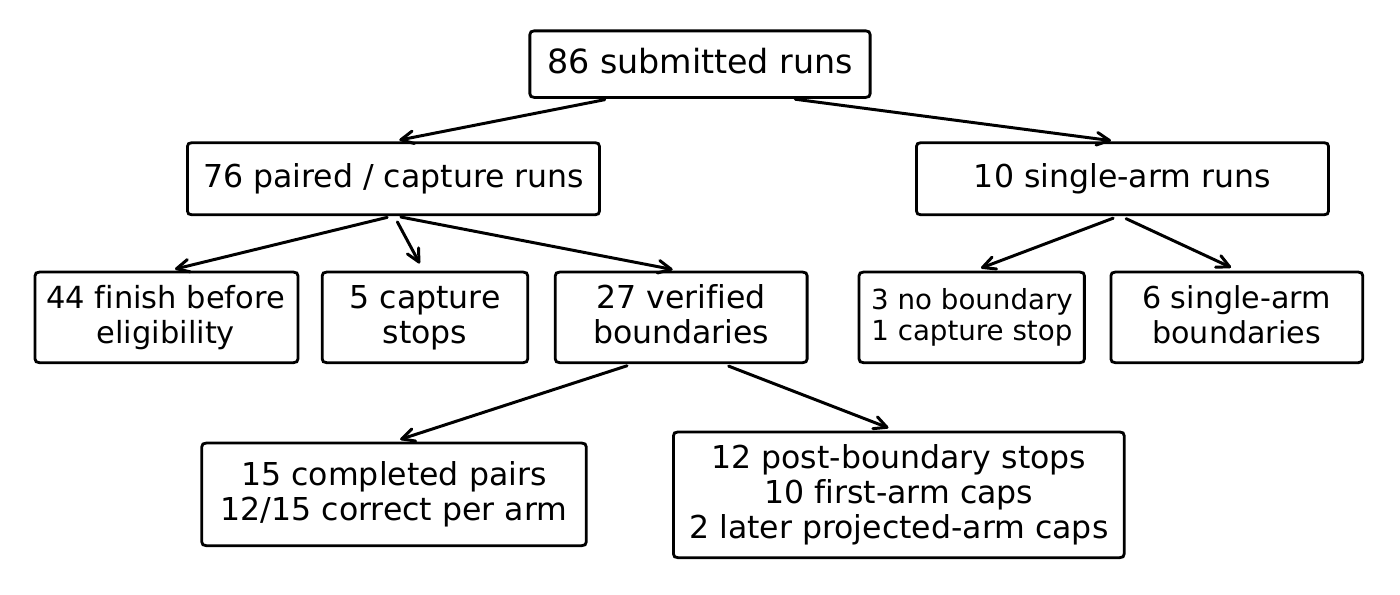
Figure 2 (the paper’s run-flow diagram): the 86 submitted runs split into 76 paired/capture and 10 single-arm integration runs. Only 27 paired/capture runs reach a boundary, then divide into 15 completed pairs and 12 stopped pairs. The key is which boundaries the complete-pair filter removes, not a rate that should be projected to other campaigns (Section 5.1). Original Figure 2 by Zhang, “Completed Pairs Hide Capped Failures,” arXiv v1, from figures/run_flow.pdf in the arXiv source archive; reused under CC BY 4.0.

Core intuition: completion order selects the pair table

Suppose both branches are allocated in advance, but whether the second runs depends on whether the first finishes. A non-completion can arise because the intervention is difficult for the agent, or because the model or tool budget is genuinely exhausted. If the runner responds to non-completion of the first arm with break, the schedule has a precise consequence: conditional on a first-arm non-completion, the companion’s observation probability is zero. This is not an ordinary missing row that can be recovered from the companion’s observed history. That region contains no companion outcomes to estimate or weight back into the analysis (Section 3.3, Equation 2, Appendix A.3).

Of the 27 paired/capture boundaries in this campaign, 15 completed both arms and 12 stopped. In ten, the first arm used its request cap and the runner did not execute its companion. In the other two, full completed first and projected later reached its cap. Initial order is hash-seeded within each source group and alternates across siblings, giving 15 F-first and 12 P-first records; this is deterministic allocation, not independent random assignment. The first-arm cap counts are 3/15 for F-first and 7/12 for P-first, but these boundary subsets contain different tasks and sources. Their difference is not a causal estimate of order (Section 3.3, Table 2, Appendix B Table 8).

Keep only the 15 completed pairs and both F and P are correct in 12/15. That looks identical. Within those pairs, however, 11 are jointly correct, two jointly incorrect, one is full-only correct, and one is projected-only correct. In the 12 stopped pairs, every record contains at least one observed cap failure; ten have an entirely unrun companion whose outcome remains unknown. The complete-pair filter removes these boundaries from its headline summary. Symmetry of 12/15 in the retained rows does not tell us whether an excluded companion would have succeeded or failed.

Why the prior approach is insufficient: a complete-pair filter cannot recover an unobservable companion

Benchmark reports often treat complete pairs as a ready-made comparison set. But if a runner’s stopping rule makes the companion impossible to observe under a particular first-arm outcome, a complete-case filter conditions on that schedule and drops both the failure and its unknown counterpart. Where the companion’s observation probability is zero, a regression on the observed first-arm result or inverse-observation weighting has no observations from which to estimate it; the latter would divide by zero. The methodological limitation is not that all paired analyses are wrong. It is that a completed-pair summary does not expose the positivity gap created by this particular schedule. Appendix A.3 also explains why adjustment for the observation process cannot supply a companion outcome that was never collected.

Known failures and unknown outcomes: a cap is a bounded failure, not permanent inability

The paper defines each outcome relative to a concrete allowance: for continuation i, let K_i = 12 be the number of new suffix requests. If no correct final answer appears within those twelve requests, the bounded outcome for that arm is 0. Using all twelve without an answer is a known failure to complete within this allowance. It does not show that the task would remain unanswered with a larger budget, nor that the model is incapable of solving it. By contrast, when the companion received no request at all, its outcome is unknown: it cannot be coded as either 0 or success (Section 4.1, Equation 4).

This distinction yields explicit counts across the 27 boundaries. Full has 14 known successes, six known failures, and seven unexecuted arms. Projected has 12 known successes, twelve known failures, and three unexecuted arms (Section 5.2, Table 3). Define the pair contrast as Y_P - Y_F. The observed success counts first contribute 12 - 14 = -2 tasks. To obtain the endpoint most adverse to P, assign P’s three unknowns to 0 and F’s seven unknowns to 1; the contrast falls by seven more tasks to -9/27. At the endpoint most favorable to P, assign P’s unknowns to 1 and F’s unknowns to 0; the contrast rises by three to +1/27. Thus the contrast in this fixed 27-task frame is bounded by [-33.3, +3.7] percentage points.

The interval means partial identification: without inventing results for unexecuted arms, it describes the minimum and maximum frame average across every binary completion of unknowns compatible with what was observed. Both endpoints can be attained by an admissible assignment. This is not a repeated-sampling confidence interval; it does not estimate sampling error for a deployment population or attach a confidence level to that population’s true contrast. It still allows P to have one more success, and it also allows P to have nine fewer. The paper can therefore reject the inference “the completed-pair tie means the whole frame is tied.” It cannot claim that projection is generally worse or noninferior outside this design (Appendix A.1, Table 3, Table 6).

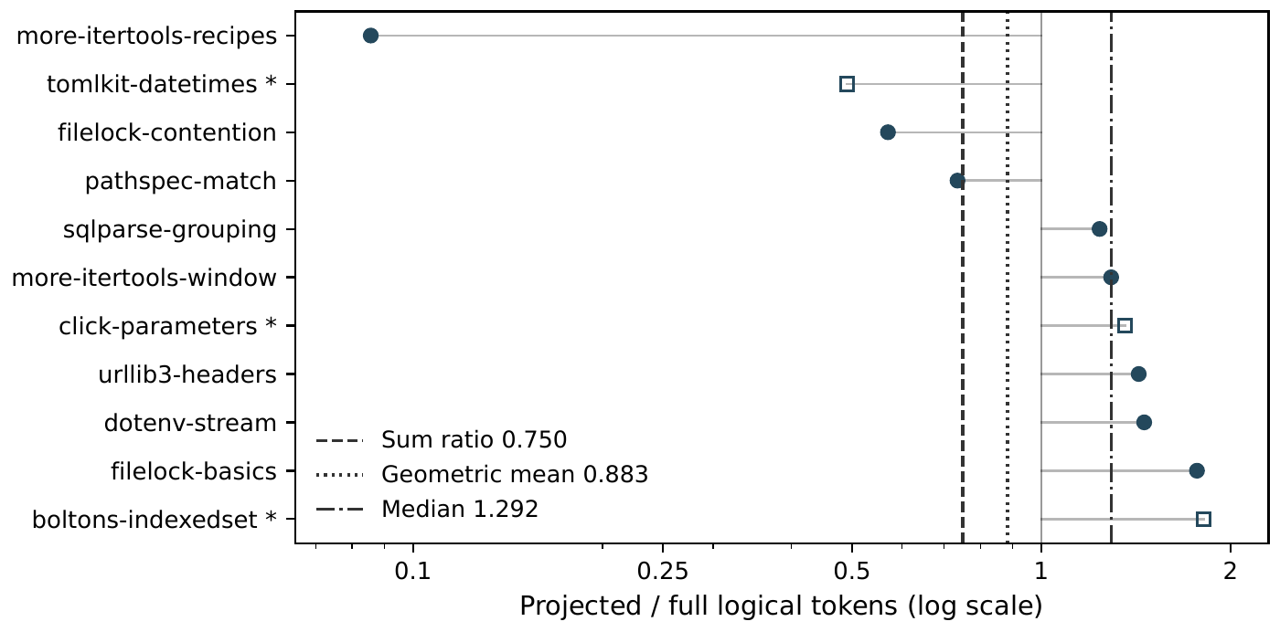
Figure 3 (the paper’s pair-ratios plot): each point is the projected/full logical-token ratio for one of the eleven pairs where both arms were correct. Dashed, dotted, and dash-dot lines mark the ratio of sums at 0.750, geometric mean at 0.883, and median at 1.292 (Section 5.4). A ratio of 1 means equal tokens; a value above 1 means P used more. Hollow markers and asterisks identify fitting cases. This figure does not establish completion rates for all 27 runs. Original Figure 3 by Zhang, “Completed Pairs Hide Capped Failures,” arXiv v1, from figures/pair_ratios.pdf in the arXiv source archive; reused under CC BY 4.0.

Fitting and outside-fitting cases: an aggregate tie can still conceal selection

The paper also studies a frozen selector that chooses which arm to run based on history bytes. A search over 36 candidate rules sets the threshold at 93,641 bytes: if a history is at least that long, choose projected; otherwise choose full. Four completed fitting pairs were used to select the threshold. Those pairs also appear in the later observed comparison, so the 17-run frame with both bounded outcomes known is not a pure held-out test (Sections 3.4, 5.3).

On the same 17 runs, always-full has three failures and 1,823,900 logical tokens. The selector also has three failures but uses 1,840,140 tokens: 16,240 more, or about 0.9%. The aggregate failure tie depends on fitting rows. Among the four fitting pairs, the selector has no failures while full has one, because projected succeeds and full fails on packaging-compatibility. The selector’s logical token total is 26.3% lower on that fitting subset.

Remove the four fitting pairs and look at the 13 outside-fitting observations. Always-full has two failures and 1,419,197 tokens; the selector has three failures and 1,541,879 tokens, or 122,682 more (about 8.6%). The additional failure is pathspec-util, where the selector chose projected and the continuation reached its cap. This split shows that the 3/17 overall tie is not evidence of a tie outside fitting. But “outside-fitting” does not mean a new, pre-registered, untouched test set; these are still observations accumulated within the same adaptive campaign (Table 4, Appendix C Table 11).

Readers should not treat the threshold or a hindsight row as a deployable policy. Using the same 17 observed runs, the paper also computes a hindsight threshold that optimizes for observed failures and token expenditure; its value happens to equal another fitting history. This is an in-sample reference for the same threshold family, not a fair forecast of future behavior or an upper bound on every possible agent improvement. In particular, moving the threshold to avoid the known pathspec-util history would be another fit to a known case, not independent confirmation.

Cost results: aggregate savings, a higher median, and more requests can coexist

The paper separately defines a fully observed success stratum J: pairs where both F and P answered correctly within the 12-request cap. Why does this set not depend on how an unexecuted companion is filled in? Every one of the twelve stopped boundaries has at least one arm known to be 0, so no such pair can belong to J under any completion of the missing outcomes. Therefore, J is fixed at eleven pairs within the 27-boundary frame, and the cost comparison within it is fully observed. This is the successful stratum under the recorded coupling; it is not a population survivor-average causal effect for future stochastic reruns (Section 4.2, Appendix A.1).

For these eleven pairs, full uses 1,267,036 logical tokens in aggregate and projected uses 949,774. The ratio of sums is 0.750, or 25% fewer aggregate tokens. But the distribution of each pair’s token ratio tells a different story: the geometric mean is 0.883, the median is 1.292, and P uses more tokens in 7/11 pairs. In this stratum, a lower aggregate and a more expensive median pair are compatible. The ratio of sums weights each pair by its full-arm token baseline, so a very expensive pair with large savings can affect the total more than a low-cost pair. The geometric mean aggregates multiplicative changes; the median identifies the middle ranked pair. They are not three tests of one interchangeable claim; they answer different questions (Equation 11, Section 5.4, Figure 3).

It also matters how concentrated the aggregate is. more-itertools-recipes uses nine suffix requests in the full continuation but only one in projected, producing the largest absolute token saving. If that one pair is left out in a sensitivity calculation, the ratio of sums changes from 0.750 to 1.077. This does not erase the paper’s prespecified primary analysis. It shows why the 25% aggregate must be read with the sample composition in view. The paper reports a two-sided sign-test reference of p = 0.55 for seven of eleven token increases, but because tasks share sources and the frame was adaptive, the authors do not treat it as a test of general harm (Appendix C).

Interaction counts add another view of the agent’s work. P uses more suffix requests in eight pairs, fewer in two, and the same number in one, for 55 versus 35 requests overall, a 57% increase. Shorter average input per request therefore does not imply fewer calls, lower wall time, or lower monetary cost to complete a task. The token report separates uncached input, cached input, and output; cached input is a subset of input and must not be counted a second time as extra tokens. In J, projected is accompanied by 89,684 more uncached input tokens, 407,680 fewer cached input tokens, and 734 more output tokens. Rewriting earlier request prefixes may change cache reuse, while continuations themselves also diverge. These records do not isolate cache change as a single causal mechanism.

Nor can the token totals be translated directly into dollars. The author’s private price schedule and invoices are unavailable, so the paper can substitute arbitrary prices for uncached input, cached input, and output in a symbolic sensitivity calculation, but cannot establish dollar savings in this campaign. The totals of 641 requests and 8,202,832 tokens for the campaign as a whole should not be mixed into the J cost comparison either: the denominators answer different questions. All reported values belong to this one campaign, not to ReVerPi or context projection as benchmark constants (Sections 4.3, 5.1, and 5.4).

Worked example: follow a complete failure trace from archive access to no final answer

The most concrete example is pathspec-util. Its history is 94,493 bytes, above the frozen selector’s 93,641-byte threshold, so the rule chooses projected. From the common prefix, full makes three suffix model requests and returns a correct answer using 84,202 suffix tokens. Projected successfully retrieves archived text: its first exact read returns content, and its second request searches and finds text. The next two exact-read attempts encounter the shared archive-call quota refusal. The model continues reading source fragments until it uses all 12 suffix requests, without a final answer.

In the recorded trace, projected uses 237,629 suffix tokens. Including the 39,539-token common prefix, full uses 123,741 logical tokens and projected uses 277,168. Projected’s average per suffix request is about 19.8k, roughly 29% below full’s 28.1k, yet P uses four times the requests and 2.82 times the suffix-token expenditure. This is the break between “fewer tokens per request” and “less total work before a task answer.”

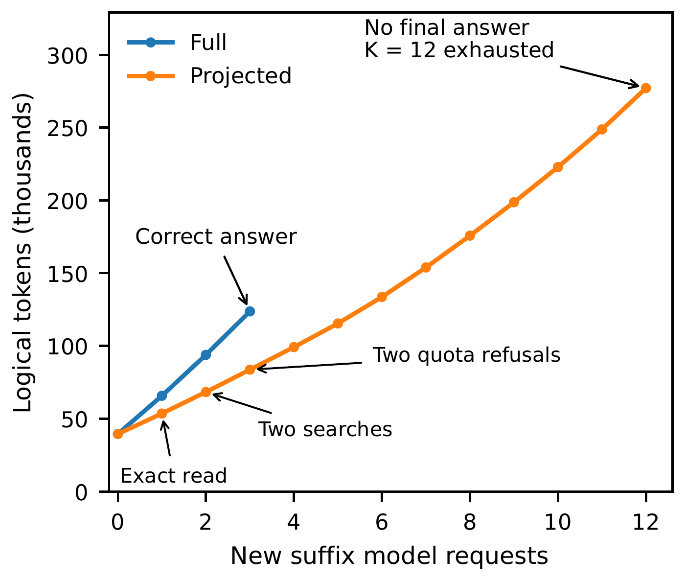
Figure 4 (the paper’s pathspec-util cost trace): both lines share the same capture prefix. Full returns a correct answer after three suffix requests. Projected successfully exact-reads and searches in its early requests, then encounters two quota refusals and continues to K = 12 without a final answer. The figure supports the claim that this recorded projected trace retrieved archive text but still failed within the cap. It does not show that the agent would necessarily fail with a larger quota or that the retrieved passages were insufficient (Section 5.5). Original Figure 4 by Zhang, “Completed Pairs Hide Capped Failures,” arXiv v1, from figures/pathspec_cost.pdf in the arXiv source archive; reused under CC BY 4.0.

This quota failure also exposes a runtime contract detail. The recovery tool returned isError: true in its result object, but the pinned Pi loop marks a tool failure only when execute throws an exception. The quota refusal therefore appeared in the model-visible output with isError=false; the short tool result was also protected from projection. The model saw refusal text, but the runtime supplied no structured error state that would force it to stop or change strategy. The paper says this error-signaling mismatch was fixed in pull request 15 after the campaign; that later repair cannot alter the already-recorded request trajectory. The trace establishes a successful archive lookup, later quota refusals, and a run that reached the cap without answering. It does not establish what would happen with a larger quota, or that search returned insufficient content (Section 5.5, Appendix D, Figure 4).

Preserve one more distinction: storage availability, tool access, and task completion are separate states. The full text can exist in an archive without the agent having read enough evidence. A successful tool call does not guarantee that more operation quota remains. If a search excerpt already contains the answer, requiring another exact read can waste quota. A failed read should remain a measured request and boundary, rather than being collapsed into “retrieval succeeded, therefore the method worked” or “a cap was reached, therefore the method can never work.”

Evidence map: what these records support, what the authors claim, and what remains unknown

Layer	Distinction to retain
Paper directly supports	The runner’s stop rule, observed states across 27 paired/capture boundaries, finite-frame bounds, the selector’s fitting split, and the cost distribution in eleven jointly successful pairs.
Author claims	Completed-pair summaries hide some bounded failures; evaluations should retain each intervention boundary and execute/report allocated continuations separately.
Not supported by the evidence	The prevalence of bias in other benchmarks, population superiority/noninferiority, dollar savings inferred from token totals, or a universal effect of projection across agent tasks.
Our engineering judgment	Map allocation, stop reason, outcome status, and estimand to auditable fields. This is an engineering synthesis, not a general standard validated by the authors.

Observed frame	Supported statement	Do not turn it into
15 completed pairs	Each arm was correct on 12/15 of the pairs retained by this filter.	Equal success across every allocated intervention.
27 paired/capture boundaries	The projected-minus-full success difference in this record is bounded from -9 to +1 tasks, keeping known cap failures separate from unknown companions.	Population superiority or noninferiority, a general rate of bias, or a model for the probability of missing outcomes.
17 runs with both outcomes known	The frozen selector and always-full each have three failures; the selector uses 0.9% more logical tokens.	A tie on unseen cases; these 17 include fitting cases.
13 outside-fitting runs	The selector has one extra failure and uses 8.6% more logical tokens than always-full.	A fully independent holdout result; these records still come from an adaptive campaign.
11 jointly correct pairs	P uses 25% fewer aggregate logical tokens, while the median pair uses 29% more and requests rise 57%.	Overall success, cost to success for all tasks, dollar savings, or a deployment expectation.

The paper’s strongest empirical contribution is connecting control flow to the estimand. If the runner stops after a first-arm cap, its schedule makes companion outcomes entirely unobservable in that region. A regression or observation adjustment on the observed first-arm result cannot conjure the counterfactual that the schedule never collected. The most information-preserving approach is to label known success, known bounded failure, and unknown separately, then report bounds over every compatible assignment for the fixed finite frame (Sections 3.3–4.2, Appendix A).

The paper does not show that all paired benchmarks are invalid. Ten first-arm caps are facts about this runner’s schedule, not a prevalence estimate for other systems; the 27 boundaries are not a random sample of an agent-task population. Order alternates by hash parity within source groups but is not independently randomized. The questions were developed adaptively from package subsets, and each arm has one stochastic continuation. The model name and usage are provider-reported proxy labels, not authentication of backend weights. The read-only source adapter has an allowlist, but is not an adversarial sandbox for the full Pi product. Historical first-decodable-JSON scoring remains primary; a stricter whole-object sensitivity adds one failure to each arm without changing the selector comparison (Section 6, Appendix C).

The appendices also examine single-arm integrations, changing history sizes for repeated tasks, threshold sensitivity, a zero-event calibration reference, source inventory, and artifact integrity. These materials help bound the case; they do not add a deployment claim to the headline. In particular, the calibration appendix’s fixed-sample formula depends on independent Bernoulli assumptions. Recomputing that formula does not give a population risk guarantee to an adaptive, complete-case campaign. Source digests support file-consistency checks; they do not prove the chronology of historical events, provider backend identity, or the actual bill (Appendices A, B, C, E, F).

Bloss0m engineering judgment: treat the runner’s stop rule as an experimental variable

The following is a Bloss0m engineering judgment drawn from the paper, not a universal benchmark standard empirically established by the authors. When designing a paired evaluation, model runner state as first-class data: each allocated arm should have an allocation ID, launch state, each relevant cap, stop reason, completion state, and indicator of whether it ran. A completed pair is one result category, not the only row permitted in the results table.

• Separate schedule from outcome. When permissions, data integrity, and environment safety allow, reserve and execute the two arms separately. If a reasonable cap, invalid environment, or revoked permission must stop an arm, preserve the unexecuted state and concrete reason; do not let its companion disappear from the denominator.
• Report opportunity alongside answers. Eligible boundaries, request opportunities, completion, correctness, failed attempts, and unknown outcomes should have separate counts. Also separate runs that never reached intervention eligibility from actual intervention boundaries, so readers do not assume every submitted run received the treatment.
• Choose the estimand before the summary. Completion within a fixed cap, correct final answer, token cost within the success stratum, per-pair median, and aggregate expenditure are different estimands. State which one matters to the decision before choosing the denominator and aggregation.
• Preserve fitting lineage for adaptive selectors. List the tasks used to select the rule, how the threshold was chosen, and whether purportedly outside-fitting samples were truly held aside in advance. Do not let a development-set tie look like independent evaluation.
• Make resource failures visible. Controller caps, archive-call quotas, provider request caps, and task deadlines should be logged separately. Send quota errors as both structured status and model-visible signals; downstream control should not have to infer a tool failure from prose alone.

In the Discussion, the author recommends executing separately both continuations already allocated at a sealed boundary rather than suppressing the companion after an ordinary first-arm cap. Revoked permission, integrity faults, and unsafe environments may still justify stopping, but unresolved outcomes should remain visible. This is the paper’s direct protocol recommendation. The allocation IDs, estimand-specific tables, and lineage model above are a Bloss0m engineering synthesis of that recommendation (Section 6).

When not to apply this paper’s conclusion directly

Do not use this case to claim that a particular context-compression method generally saves tokens or money. Its cost figures are limited to eleven jointly successful pairs, the aggregate is highly influenced by one pair, and the token price schedule and invoices are unavailable. Do not treat -9/+1 as an expected difference for a new product: the finite-frame bound belongs to 27 recorded boundaries. If a runner stops for safety, revoked permission, or data corruption rather than ordinary resource exhaustion, blindly forcing the companion to run may violate real constraints; preserve the unobserved state and explain it under the study’s comparability and safety policy. Finally, without the same captured prefix, request cap, task protocol, and historical private provider records, you cannot claim to reproduce the author’s provider-backed campaign.

Artifacts and reproducibility

As of 2026-09-29, the authors’ ReVer_Pi GitHub repository publicly contains MIT-licensed code, tests, pinned dependency files, mock configurations, and scripts/offline-smoke.sh. The README describes this path as a protocol-only mock running from a loopback gateway through a session and Pi extension to the ledger, without API credentials or external provider calls. It is useful for checking repository wiring; it does not reproduce model performance or the paper’s 86-run campaign. A real-provider path is a separate, explicitly configured step involving paid API calls.

The arXiv v1 source archive also includes anc/ analysis inputs, scripts, an example task and observation, and data digests for recalculating the published tables and figures; its figures/ directory contains five original figures. It does not include the complete raw provider request/response archive, private configuration, session/ledger databases, or invoices. The paper says its repository and supplement reproduce the reported calculations; that does not mean they independently replay the private provider service. All experimental figures in this reading are author-reported; no independent provider-backed rerun was performed. Downloadable code and fully reproducible study results are two different claims (Section 1, Appendix E; repository README and Getting Started).

Further reading

• SWE-Bench ProMax: reading agent benchmark trajectories and cost: continue with how the evaluation frame and agent outcome affect reported numbers.
• Tool Calls Can Succeed While the Workflow Fails: take unknown outcomes from benchmark runners to external effects and runtime contracts.
• SilentProbe: Silent Failures in Agent Tool APIs: ask whether a tool response itself is reliable; this paper focuses on scheduling and an unobserved branch beyond the response.

Three things to remember

1. Technical idea: A completed-pair filter is not just a tidy table convention. When the runner suppresses a companion after first-arm non-completion, it selects which outcomes are observed.
2. Evidence: The 15 completed pairs in this campaign show 12/15 correct answers per arm. With all 27 boundaries retained, projected-minus-full success is bounded from -9 to +1 tasks.
3. Adoption boundary: Aggregate token reduction can coexist with a higher median pair cost, more requests, known cap failures, and unknown companions. These are distinct facts within this campaign, not universal laws about agents.

Primary sources

• Guangzhe Zhang, “Completed Pairs Hide Capped Failures: A ReVerPi Case Study of Selective Context Projection,” arXiv:2609.31381v1, 2026-09-25. Main anchors: Sections 3.1–3.4, 4.1–4.3, 5.1–5.6, and 6; Figures 2–4; Tables 1–6 and 8–12; Equations 2, 4–5, and 8–11; Appendices A–F.
• arXiv v1 PDF and source archive, licensed on the source page under CC BY 4.0.
• ReVer_Pi repository and its MIT license.